CS6015: Linear Algebra and Random Processes
Lecture 37: Exponential families of distributions
Learning Objectives
What are exponential families ?
Why do we care about them?
What are exponential families?
A set of probability distributions whose pmf(discrete case) or pdf (continuous case) can be expressed in the following form
f_{X}(x|\theta) = h(x) exp[\eta(\theta)\cdot T(x) - A (\theta)]
T, h: known~functions~of~x
\eta, A: known~functions~of~\theta
\theta: parameter
p
n,p
the support of \(f_X(x|\theta)\) should not depend on \(\theta\)
the support depends on \(n\)
Recap: Parameters
\mu, \sigma
Normal
Bernoulli
Binomial
Questions of Interest
Are there any popular families that we care about?
Why do we care about this form?
Many! (we will see some soon)
This form has some useful properties! (we will see some of these properties soon)
f_{X}(x|\theta) = h(x) exp[\eta(\theta)\cdot T(x) - A (\theta)]
Example 1: Bernoulli Distribution
f_{X}(x|\theta) = h(x) exp[\eta(\theta)\cdot T(x) - A (\theta)]
p_{X}(x) = p^x(1-p)^{1-x}
\theta = p
= \exp(\log(p^x(1-p)^{1-x}))
= \exp(\log(p^x(1-p)^{1-x}))
\exp(k) = e^k
= \exp(\log p^x + \log (1-p)^{1-x})
= \exp(x\log p + (1-x)\log (1-p))
= \exp(x\log p -x\log (1-p) + \log (1-p))
= \exp(\log \frac{p}{1-p}x + \log (1-p))
h(x)=1
\eta(p)=\log \frac{p}{1-p}
T(x) = x
A(p) = -log(1-p)
Example 2: Binomial Distribution
only if \(n\) is known/fixed & hence not a parameter
p_{X}(x) = {n \choose x} p^x(1-p)^{n-x}
X = \{0,1,2,\dots, N\}
=\exp(\log({n \choose x} p^x(1-p)^{n-x}))
=\exp(\log{n \choose x} + x\log p + (n-x)\log(1-p))
=\exp(\log{n \choose x} + \log \frac{p}{(1-p)}x + n\log(1-p))
={n \choose x}\exp(\log \frac{p}{(1-p)}x + n\log(1-p))
h(x)=1
\eta(p)=\log \frac{p}{1-p}
T(x) = x
A(p) = -nlog(1-p)
f_{X}(x|\theta) = h(x) exp[\eta(\theta)\cdot T(x) - A (\theta)]
Example 3: Normal Distribution
Two parameters: \(\mu, \sigma\)
f_X(x) = \frac{1}{\sqrt{2 \pi}\sigma} \exp(\frac{-(x-\mu)^2}{2\sigma^2})
= \frac{1}{\sqrt{2 \pi}}\exp(-\log\sigma) \exp(-\frac{x^2 -2x\mu + \mu^2}{2\sigma^2})
= \frac{1}{\sqrt{2 \pi}}\exp(\frac{x\mu}{\sigma^2} + \frac{x^2}{-2\sigma^2} - \frac{\mu}{2\sigma^2} - \log \sigma)
= \frac{1}{\sqrt{2 \pi}}\exp(\begin{bmatrix}\frac{\mu}{\sigma^2} & -\frac{1}{2\sigma^2} \end{bmatrix}\begin{bmatrix}x \\ x^2 \end{bmatrix} - (\frac{\mu}{2\sigma^2} - \log \sigma))
h(x)=1
\eta(\mu, \sigma^2)=\begin{bmatrix}\frac{\mu}{\sigma^2} & -\frac{1}{2\sigma^2} \end{bmatrix}^\top
T(x) = \begin{bmatrix}x & x^2 \end{bmatrix}^\top
A(\mu, \sigma^2) = \frac{\mu}{2\sigma^2} - \log \sigma
dot product
dim. of \(\eta(\theta)\) is equal to number of parameters
f_{X}(x|\theta) = h(x) exp[\sum_i\eta_i(\theta).T_i(x) - A (\theta)]
f_{X}(x|\theta) = h(x) exp[\eta(\theta)\cdot T(x) - A (\theta)]
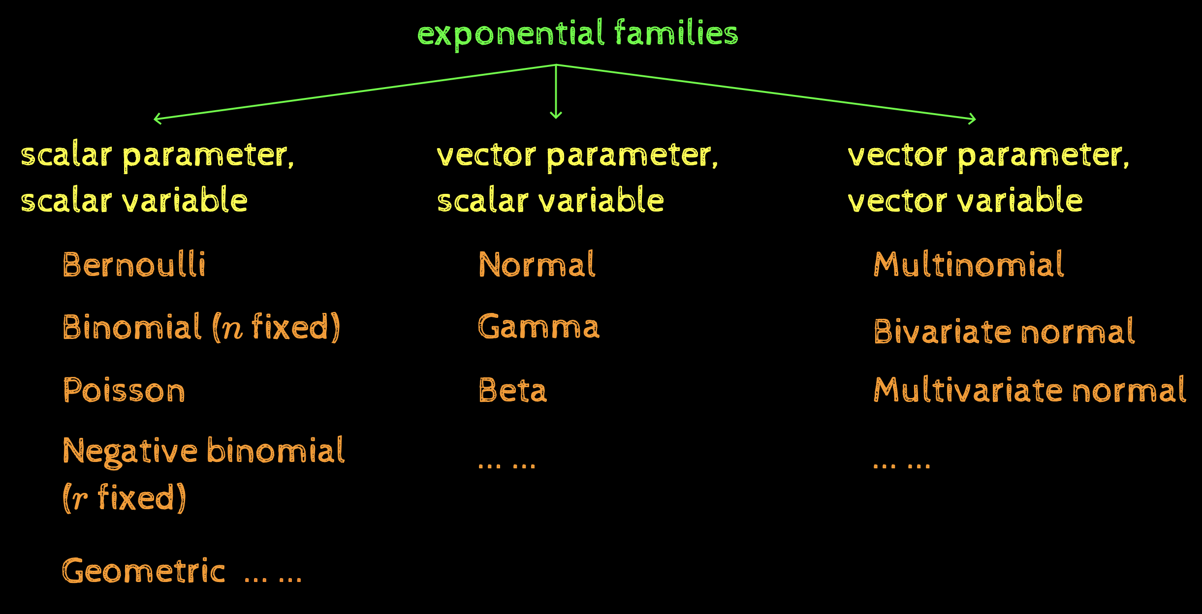
The bigger picture
exponential families
scalar parameter, scalar variable
vector parameter, scalar variable
vector parameter, vector variable
Bernoulli
Binomial (\(n\) fixed)
Poisson
Negative binomial (\(r\) fixed)
Geometric
... ...
Normal
Gamma
Beta
Multinomial
Bivariate normal
... ...
Multivariate normal
... ...
f_{X}(x|\theta) = h(x) exp[\eta(\theta)\cdot T(x) - A (\theta)]
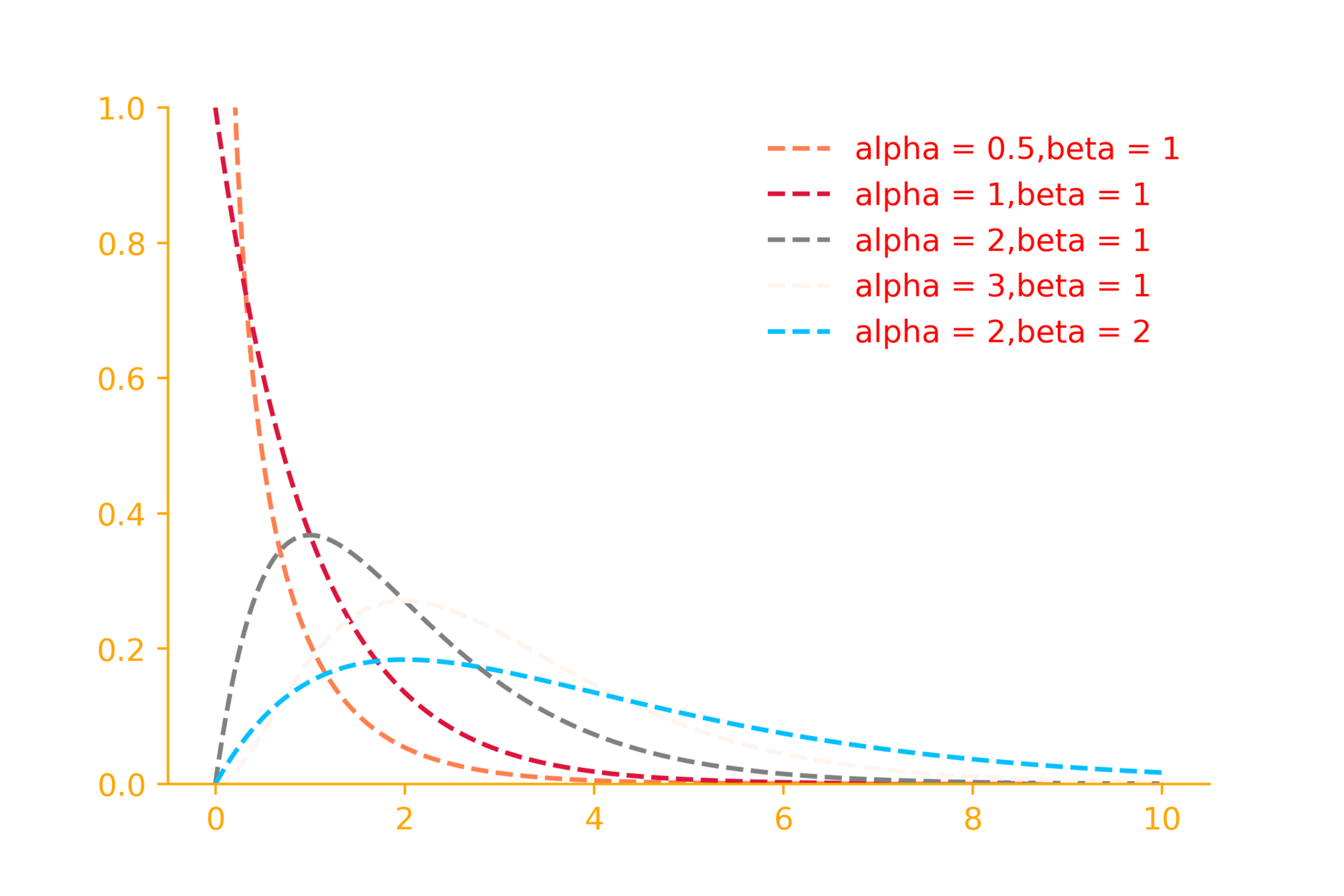
The gamma distribution
Why do families matter?
f(x) = \frac{\beta^\alpha}{\Gamma(\alpha)}x^{(\alpha - 1)}e^{-\beta x}
\Gamma(\alpha) = (\alpha - 1)!
\alpha = shape~parameter
\beta = rate~parameter
import matplotlib.pyplot as plt
from scipy.stats import gamma
import numpy as np

x = np.linspace(0, 10, 500)
alpha = 3
beta = 1
rv = gamma(alpha, loc = 0., scale = 1/beta)

plt.plot(x, rv.pdf(x))
Example 4: Bivariate normal
f_{X,Y}(x,y) = \frac{1}{2 \pi |\Sigma|^{\frac{1}{2}}}\exp(-\frac{1}{2}(\mathbf{x} - \mu)^T\Sigma^{-1}(\mathbf{x} - \mu))
= \frac{1}{2 \pi} |\Sigma|^{-\frac{1}{2}}\exp(-\frac{1}{2}(\mathbf{x} - \mu)^T\Sigma^{-1}(\mathbf{x} - \mu))
= \frac{1}{2 \pi} \exp(-\frac{1}{2}(\mathbf{x}^\top\Sigma^{-1}\mathbf{x} + \mu^\top\Sigma^{-1}\mu - 2\mu^\top\Sigma^{-1}\mathbf{x} + \ln|\Sigma|))
\mathbf{x} = [x~~y]^\top
f_{X}(x|\theta) = h(x) exp[\eta(\theta)\cdot T(x) - A (\theta)]
= \frac{1}{2 \pi} \exp(-\frac{1}{2}\mathbf{x}^\top\Sigma^{-1}\mathbf{x} + \mu^\top\Sigma^{-1}\mathbf{x} -\frac{1}{2} \mu^\top\Sigma^{-1}\mu -\frac{1}{2} \ln|\Sigma|)
= \frac{1}{2 \pi} \exp(-\frac{1}{2}vec(\Sigma^{-1})^\top vec(\mathbf{x}\mathbf{x}^\top) + \mu^\top\Sigma^{-1}\mathbf{x} -\frac{1}{2} \mu^\top\Sigma^{-1}\mu -\frac{1}{2} \ln|\Sigma|)
h(x)=\frac{1}{2\pi}
\eta(\mu, \Sigma)=\begin{bmatrix}
\Sigma^{-1}\mu \\
-\frac{1}{2}vec(\Sigma^{-1})
\end{bmatrix}
T(x) =\begin{bmatrix}
\mathbf{x} \\
vec(\mathbf{x}\mathbf{x}^\top)
\end{bmatrix}
A(\mu, \Sigma) = \frac{1}{2} (\mu^\top\Sigma^{-1}\mu + \ln|\Sigma|)
Example 5: Multivariate normal
Try on your own
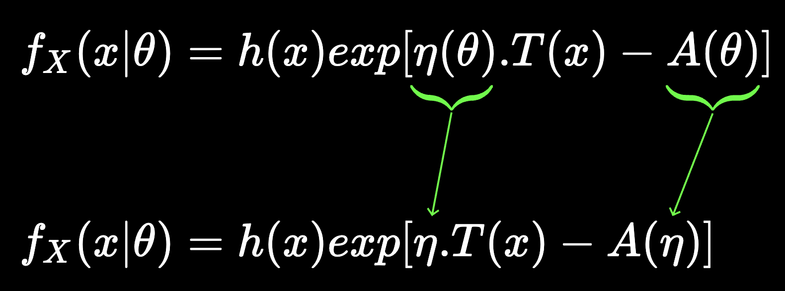
Natural parameterisation
f_{X}(x|\theta) = h(x) exp[\eta(\theta).T(x) - A (\theta)]
f_{X}(x|\theta) = h(x) exp[\eta.T(x) - A (\eta)]
\underbrace{~~~~~~~}
\underbrace{~~~~~~~~}
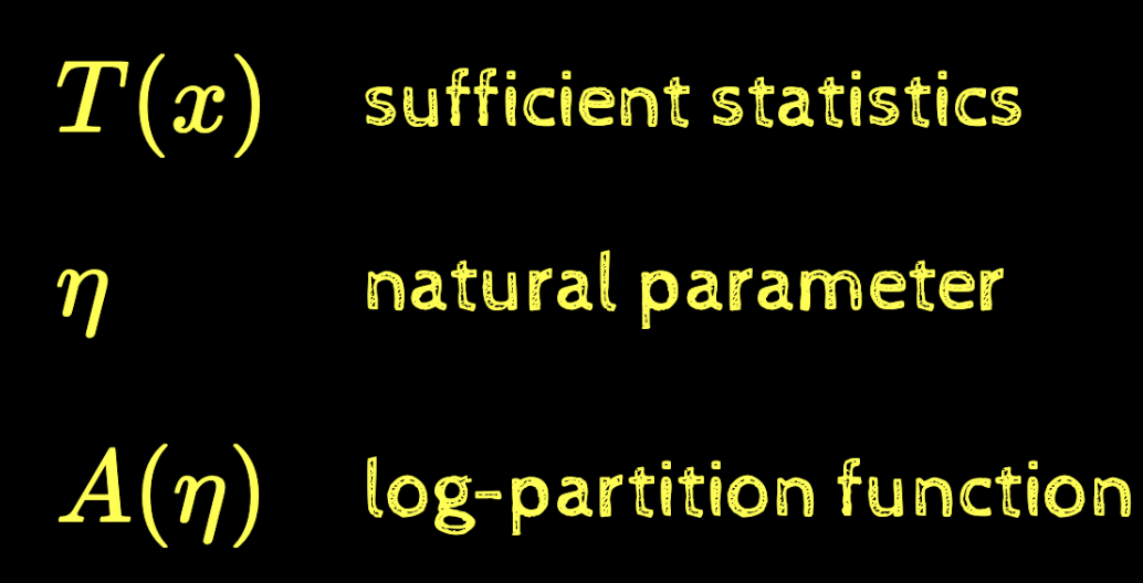
sufficient statistics
T(x)
\eta
natural parameter
A(\eta)
log-partition function
Revisiting the examples
Bernoulli
p(x)= \exp(\log \frac{p}{1-p}x + \log (1-p))
h(x)=1
\eta(p)=\log \frac{p}{1-p}
T(x) = x
A(p) = -\log(1-p)
Let~\eta=\log \frac{p}{1-p}
then~A(\eta)=\log (1+e^\eta)
p(x)= \exp(\eta x - \log (1+e^\eta))
Revisiting the examples
Binomial
p(x)={n \choose x}\exp(\log \frac{p}{(1-p)}x + n\log(1-p))
h(x)=1
\eta(p)=\log \frac{p}{1-p}
T(x) = x
A(p) = -n\log(1-p)
Let~\eta=\log \frac{p}{1-p}
then~A(\eta)=n\log (1+e^\eta)
p(x)= \exp(\eta x - n\log (1+e^\eta))
Revisiting the examples
Normal
f(x) = \frac{1}{\sqrt{2 \pi}}\exp(\begin{bmatrix}\frac{\mu}{\sigma^2} & -\frac{1}{2\sigma^2} \end{bmatrix}\begin{bmatrix}x \\ x^2 \end{bmatrix} - (\frac{\mu}{2\sigma^2} - \log \sigma))
h(x)=1
\eta(\mu, \sigma^2)=\begin{bmatrix}\frac{\mu}{\sigma^2} & -\frac{1}{2\sigma^2} \end{bmatrix}^\top
T(x) = \begin{bmatrix}x & x^2 \end{bmatrix}^\top
A(\mu, \sigma^2) = \frac{\mu}{2\sigma^2} - \log \sigma
\eta = [\eta_1, \eta_2] = [\frac{\mu}{\sigma^2}, -\frac{1}{2\sigma^2}]
A(\eta) = -\frac{\eta_1^2}{4\eta_2} - \frac{1}{2}\log(-2\eta_2)
Revisiting the examples
Bivariate normal
f(x) = \frac{1}{2 \pi} \exp(-\frac{1}{2}vec(\Sigma^{-1})^\top vec(\mathbf{x}\mathbf{x}^\top) + \mu^\top\Sigma^{-1}\mathbf{x} -\frac{1}{2} \mu^\top\Sigma^{-1}\mu -\frac{1}{2} \ln|\Sigma|)
h(x)=\frac{1}{2\pi}
\eta(\mu, \Sigma)=\begin{bmatrix}
\Sigma^{-1}\mu \\
-\frac{1}{2}vec(\Sigma^{-1})
\end{bmatrix}
T(x) =\begin{bmatrix}
\mathbf{x} \\
vec(\mathbf{x}\mathbf{x})^\top
\end{bmatrix}
A(\mu, \Sigma) = \frac{1}{2} (\mu^\top\Sigma^{-1}\mu + \ln|\Sigma|)
Try on your own
Revisiting the examples
Multivariate norm.
Try on your own
The log-partition function
f_{X}(x) = h(x) exp[\eta.T(x) - A (\eta)]
= h(x) exp(\eta.T(x))exp(- A (\eta))
= g(\eta) h(x) exp(\eta.T(x))
g(\eta) = exp(-A(\eta))
A(\eta) = -\log g(\eta)
\underbrace{~~~~~~~~~~~~~~~~~~~~~~~~~~~~}
p(x) = h(x) exp(\eta.T(x))
the kernel - encoding all dependencies on \(x\)
We can convert the kernel to a probability density function by normalising it
The log-partition function
f_{X}(x) = \frac{1}{Z}p(x)
g(\eta) = exp(-A(\eta))
A(\eta) = -\log g(\eta)
p(x) = h(x) exp(\eta.T(x))
the kernel - encoding all dependencies on \(x\)
Z = \int_x p(x) dx
\(Z\) is called the partition function
Z = \int_x h(x) exp(\eta.T(x)) dx
1 = \int_x f_x(x) dx
= \int_x g(\eta) h(x) exp(\eta.T(x)) dx
= g(\eta) \int_x h(x) exp(\eta.T(x)) dx
= g(\eta) Z
The log-partition function
g(\eta) = exp(-A(\eta))
A(\eta) = -\log g(\eta)
p(x) = h(x) exp(\eta.T(x))
the kernel - encoding all dependencies on \(x\)
1 = g(\eta) Z
g(\eta) = \frac{1}{Z}
\log g(\eta) = \log \frac{1}{Z}
-A(\eta) = - \log Z
A(\eta) = \log Z
(log partition)
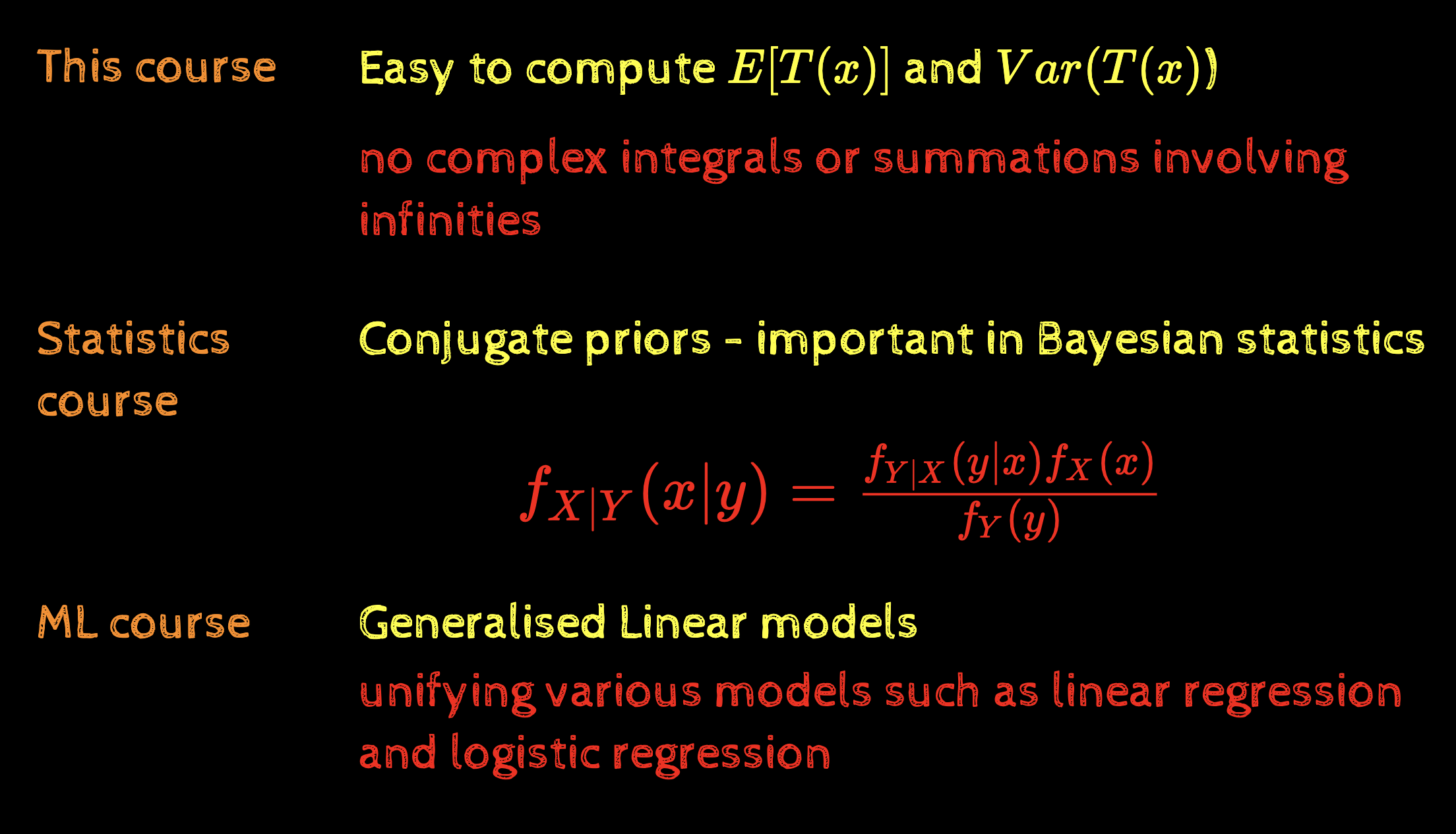
Properties (why do we care?)
Easy to compute \(E[T(x)]\) and \(Var(T(x)\))
no complex integrals or summations involving infinities
Conjugate priors - important in Bayesian statistics
This course
Statistics course
f_{X|Y}(x|y) = \frac{f_{Y|X}(y|x)f_{X}(x)}{f_{Y}(y)}
ML course
Generalised Linear models
unifying various models such as linear regression and logistic regression
Properties (why do we care?)
Easy to compute \(E[T(x)]\) and \(Var(T(x)\))
no complex integrals or summations involving infinities
It can be shown that
E[T_i(x)] = \frac{\partial A(\eta)}{\partial \eta_i}
Var[T_i(x)] = \frac{\partial^2 A(\eta)}{\partial \eta_i^2}
Proof left as an exercise
Recap: Normal dist.
\eta = [\frac{\mu}{\sigma^2}, -\frac{1}{2\sigma^2}]
T(x) = [x, x^2]
A(\eta) = -\frac{\eta_1^2}{4\eta_2} - \frac{1}{2}\log(-2\eta_2)
Alternative forms
f_{X}(x) = h(x) \exp[\eta(\theta)\cdot T(x) - A (\theta)]
f_{X}(x) = h(x) g(\theta)\exp[\eta(\theta)\cdot T(x)]
g(\theta) = \exp[-A(\theta)]
f_{X}(x) = \exp[\eta(\theta)\cdot T(x) - A(\theta) + B(x)]
B(x) = \log(h(x))
Summary
E[T_i(x)] = \frac{\partial A(\eta)}{\partial \eta_i}
Var[T_i(x)] = \frac{\partial^2 A(\eta)}{\partial \eta_i^2}
CS6015: Lecture 37
By Mitesh Khapra
CS6015: Lecture 37
Lecture 37: The exponential family of distributions


