
Slides based on the book:
\(F_0 = 0, F_1 = 1\)
\(F_{n+2} = F_{n+1} + F_n\) for \(n = 0,1,2,\ldots\)
\(F_0, F_1, F_2, \ldots \)
#1. Fibonacci Numbers, Quickly
The Fibonacci numbers were first described in Indian mathematics, as early as 200 BC in work by Pingala on enumerating possible patterns of Sanskrit poetry formed from syllables of two lengths.
Hemachandra (c. 1150) is credited with knowledge of the sequence as well, writing that "the sum of the last and the one before the last is the number ... of the next mātrā-vṛtta."

\(\underbrace{\left(\begin{array}{cc}\star & \star \\\star & \star\end{array}\right)}_{M}\left(\begin{array}{c}F_{n+1} \\F_n\end{array}\right) = \left(\begin{array}{c}F_{n+2} \\F_{n+1}\end{array}\right)\)
#1. Fibonacci Numbers, Quickly
\(\underbrace{\left(\begin{array}{cc}{\color{IndianRed}\star} & {\color{IndianRed}\star} \\\star & \star\end{array}\right)}_{M}\left(\begin{array}{c}F_{n+1} \\F_n\end{array}\right) = \left(\begin{array}{c}F_{n+2} \\F_{n+1}\end{array}\right)\)
#1. Fibonacci Numbers, Quickly
\(\underbrace{\left(\begin{array}{cc}{\color{IndianRed}1} & {\color{IndianRed}1} \\\star & \star\end{array}\right)}_{M}\left(\begin{array}{c}F_{n+1} \\F_n\end{array}\right) = \left(\begin{array}{c}F_{n+2} \\F_{n+1}\end{array}\right)\)
#1. Fibonacci Numbers, Quickly
\(\underbrace{\left(\begin{array}{cc}{\color{IndianRed}1} & {\color{IndianRed}1} \\{\color{DodgerBlue}\star} & {\color{DodgerBlue}\star}\end{array}\right)}_{M}\left(\begin{array}{c}F_{n+1} \\F_n\end{array}\right) = \left(\begin{array}{c}F_{n+2} \\F_{n+1}\end{array}\right)\)
#1. Fibonacci Numbers, Quickly
\(\underbrace{\left(\begin{array}{cc}{\color{IndianRed}1} & {\color{IndianRed}1} \\{\color{DodgerBlue}1} & {\color{DodgerBlue}0}\end{array}\right)}_{M}\left(\begin{array}{c}F_{n+1} \\F_n\end{array}\right) = \left(\begin{array}{c}F_{n+2} \\F_{n+1}\end{array}\right)\)
#1. Fibonacci Numbers, Quickly
\(\underbrace{\left(\begin{array}{cc}{\color{IndianRed}1} & {\color{IndianRed}1} \\{\color{DodgerBlue}1} & {\color{DodgerBlue}0}\end{array}\right)}_{M}\left(\begin{array}{c}F_{n+1} \\F_n\end{array}\right) = \left(\begin{array}{c}F_{n+2} \\F_{n+1}\end{array}\right)\)
\(M\left(\begin{array}{c}F_{n+1} \\F_n\end{array}\right)=\left(\begin{array}{c}F_{n+2} \\F_{n+1}\end{array}\right)\)
#1. Fibonacci Numbers, Quickly
\(\underbrace{\left(\begin{array}{cc}{\color{IndianRed}1} & {\color{IndianRed}1} \\{\color{DodgerBlue}1} & {\color{DodgerBlue}0}\end{array}\right)}_{M}\left(\begin{array}{c}F_{n+1} \\F_n\end{array}\right) = \left(\begin{array}{c}F_{n+2} \\F_{n+1}\end{array}\right)\)
\(M\left(\begin{array}{c}1 \\0\end{array}\right)=\left(\begin{array}{c}F_{2} \\F_{1}\end{array}\right)\)
\(M\left(\begin{array}{c}F_2 \\F_1\end{array}\right)=\left(\begin{array}{c}F_{3} \\F_{2}\end{array}\right)\)
#1. Fibonacci Numbers, Quickly
\(\underbrace{\left(\begin{array}{cc}{\color{IndianRed}1} & {\color{IndianRed}1} \\{\color{DodgerBlue}1} & {\color{DodgerBlue}0}\end{array}\right)}_{M}\left(\begin{array}{c}F_{n+1} \\F_n\end{array}\right) = \left(\begin{array}{c}F_{n+2} \\F_{n+1}\end{array}\right)\)
\(M\left(\begin{array}{c}1 \\0\end{array}\right)=\left(\begin{array}{c}F_{2} \\F_{1}\end{array}\right)\)
\(M{\color{Orange}\left(\begin{array}{c}F_2 \\F_1\end{array}\right)}=\left(\begin{array}{c}F_{3} \\F_{2}\end{array}\right)\)
#1. Fibonacci Numbers, Quickly
\(\underbrace{\left(\begin{array}{cc}{\color{IndianRed}1} & {\color{IndianRed}1} \\{\color{DodgerBlue}1} & {\color{DodgerBlue}0}\end{array}\right)}_{M}\left(\begin{array}{c}F_{n+1} \\F_n\end{array}\right) = \left(\begin{array}{c}F_{n+2} \\F_{n+1}\end{array}\right)\)
\(M\left(\begin{array}{c}1 \\0\end{array}\right)=\left(\begin{array}{c}F_{2} \\F_{1}\end{array}\right)\)
\(M \cdot {\color{Orange}M \left(\begin{array}{c}1 \\0\end{array}\right)}=\left(\begin{array}{c}F_{3} \\F_{2}\end{array}\right)\)
#1. Fibonacci Numbers, Quickly
\(\underbrace{\left(\begin{array}{cc}{\color{IndianRed}1} & {\color{IndianRed}1} \\{\color{DodgerBlue}1} & {\color{DodgerBlue}0}\end{array}\right)}_{M}\left(\begin{array}{c}F_{n+1} \\F_n\end{array}\right) = \left(\begin{array}{c}F_{n+2} \\F_{n+1}\end{array}\right)\)
\(M\left(\begin{array}{c}1 \\0\end{array}\right)=\left(\begin{array}{c}F_{2} \\F_{1}\end{array}\right)\)
\(M^2\left(\begin{array}{c}1 \\0\end{array}\right)=\left(\begin{array}{c}F_{3} \\F_{2}\end{array}\right)\)
#1. Fibonacci Numbers, Quickly
\(\underbrace{\left(\begin{array}{cc}{\color{IndianRed}1} & {\color{IndianRed}1} \\{\color{DodgerBlue}1} & {\color{DodgerBlue}0}\end{array}\right)}_{M}\left(\begin{array}{c}F_{n+1} \\F_n\end{array}\right) = \left(\begin{array}{c}F_{n+2} \\F_{n+1}\end{array}\right)\)
\(M\left(\begin{array}{c}1 \\0\end{array}\right)=\left(\begin{array}{c}F_{2} \\F_{1}\end{array}\right)\)
\(M^n\left(\begin{array}{c}1 \\0\end{array}\right)=\left(\begin{array}{c}F_{n+1} \\F_{n}\end{array}\right)\)
#1. Fibonacci Numbers, Quickly
\(M^n\left(\begin{array}{c}1 \\0\end{array}\right)=\left(\begin{array}{c}F_{n+1} \\F_{n}\end{array}\right)\)
#1. Fibonacci Numbers, Quickly
\(\underbrace{M \longrightarrow M^{2} \longrightarrow M^{4} \longrightarrow M^{8} \longrightarrow M^{16} \longrightarrow M^{32} \longrightarrow \cdots}_{}\)
repeated squaring
\(\mathcal{O}(\log_2 n)\) multiplications of \(2 \times 2\) matrices.
#1. Fibonacci Numbers, Quickly
\(\underbrace{M \longrightarrow M^{2} \longrightarrow M^{4} \longrightarrow M^{8} \longrightarrow M^{16} \longrightarrow M^{32} \longrightarrow \cdots}_{}\)
repeated squaring
\(\mathcal{O}(\log_2 n)\) multiplications of \(2 \times 2\) matrices.
\(M^n = M^{(2^{k_1} + 2^{k_2} + \cdots + 2^{k_\ell})} = M^{2^{k_1}} M^{2^{k_2}} \cdots M^{2^{k_\ell}} \)
\(\mathcal{O}(\log_2 n)\) multiplications of \(2 \times 2\) matrices.
#1. Fibonacci Numbers, Quickly
If we want to compute the Fibonacci numbers by this method, we have to be careful, since the \(F_n\) grow very fast.
#1. Fibonacci Numbers, Quickly
As we will see later, the number of decimal digits of \(F_n\) is of order \(n\).
Thus we must use multiple precision arithmetic, and so the arithmetic operations will be relatively slow.
#1. Fibonacci Numbers, Quickly
#2. Fibonacci Numbers, The Formula
Consider the vector space of all infinite sequences:
\((u_0, u_1, u_2, \ldots )\)
...with coordinate-wise addition and multiplication by real numbers.
In this space we define a subspace \(\mathcal{W}\) of all sequences satisfying the equation:
\(u_{n+2} = u_{n+1}+u_n\) for all \(n = 0, 1, ...\)
Easy to verify: \(\mathcal{W}\) is a subspace.
Claim: \(dim(\mathcal{W}) = 2\).
Observe that \((0,1,1,2,3,\ldots)\) and \((1,0,1,1,2,\ldots)\) is a basis.
Goal. Find a closed-form formula for \(F_n\).
\(= (0,1,1,2,3,5,8,13,21,\ldots)\)
\(= (\ldots,\alpha^n,\ldots)\)
\(= (\ldots,\beta^n,\ldots)\)
=
+
\(\mathcal{W}\)
#2. Fibonacci Numbers, The Formula
\((\tau^0,\tau^1,\tau^2,\tau^3,\cdots) \in \mathcal{W} \)
\(\tau^k = \tau^{k-1}+\tau^{k-2}\)
\(\tau^2 = \tau+1\)
\(\tau_{1,2}=(1 \pm \sqrt{5}) / 2\)
\(\alpha=(1 + \sqrt{5}) / 2\)
\(\beta=(1 - \sqrt{5}) / 2\)
#2. Fibonacci Numbers, The Formula
=
+
\(F = c \cdot (\alpha^0,\alpha^1,\alpha^2,\alpha^3,\cdots) + d \cdot (\beta^0,\beta^1,\beta^2,\beta^3,\cdots)\)
\(0 = c + d\)
\(1 = c\alpha + d\beta\)
\(d = 1/(\beta -\alpha)\)
\(c = 1/(\alpha -\beta)\)
#2. Fibonacci Numbers, The Formula
#2. Fibonacci Numbers, The Formula
\(F_n = c \cdot \alpha^n + d \cdot \beta^n\)
\(d = 1/(\beta -\alpha)\)
\(c = 1/(\alpha -\beta)\)
\(\alpha=(1 + \sqrt{5}) / 2\)
\(\beta=(1 - \sqrt{5}) / 2\)
\(F_n = \frac{1}{\sqrt{5}} \cdot \left[ \left( \frac{1+\sqrt{5}}{2} \right)^n - \left( \frac{1-\sqrt{5}}{2} \right)^n \right] \)
#2. Fibonacci Numbers, The Formula
\(F_n = \left\lfloor \frac{1}{\sqrt{5}} \cdot \left( \frac{1+\sqrt{5}}{2} \right)^n \right\rfloor \)
Exercise 1. Show that:
Exercise 2. Use this method to work out a closed form for:
\(y_{n+2}=2 y_{n+1}-y_n\)
(Source: generatingfunctionology, Wilf;
h/t Matthew Drescher and John Azariah for a fun Twitter discussion on this.)
#3. The Clubs of OddTown
There are \(n\) citizens living in Oddtown.
Their main occupation was forming various clubs,
which at some point started threatening the very survival of the city.
⚠️ There could be as many as \(2^n\) distinct clubs!
(Well, \(2^n - 1\) if you would prefer to exclude the empty club.)
In order to limit the number of clubs, the city council decreed the following innocent-looking rules:
(1) Each club has to have an odd number of members.
(2) Every two clubs must have an even number of members in common.
#3. The Clubs of OddTown
There are \(n\) citizens living in Oddtown.
(1) Each club has to have an odd number of members.
(2) Every two clubs must have an even number of members in common.
Under these rules, it is impossible to form more than \(n\) clubs.
Example: \(\{\{1\},\{2\}, \ldots, \{n\}\}\).
(The Singletons Clubs.)
Example: \(\{\{1,2,3\},\{1,2,4\}, \ldots, \{1,2,n\}\}\).
(Where 1 and 2 are popular.)
#3. The Clubs of OddTown
There are \(n\) citizens living in Oddtown.
(1) Each club has to have an odd number of members.
(2) Every two clubs must have an even number of members in common.
Under these rules, it is impossible to form more than \(n\) clubs.
subsets of \([n]\)
vectors in \(n\)-dimensional space
#3. The Clubs of OddTown
There are \(n\) citizens living in Oddtown.
(1) Each club has to have an odd number of members.
(2) Every two clubs must have an even number of members in common.
Under these rules, it is impossible to form more than \(n\) clubs.
sets that satisfy (1) & (2)
linearly independent vectors
#3. The Clubs of OddTown
There are \(n\) citizens living in Oddtown.
(1) Each club has to have an odd number of members.
(2) Every two clubs must have an even number of members in common.
Under these rules, it is impossible to form more than \(n\) clubs.
#3. The Clubs of OddTown
There are \(n\) citizens living in Oddtown.
(1) Each club has to have an odd number of members.
(2) Every two clubs must have an even number of members in common.
Under these rules, it is impossible to form more than \(n\) clubs.
1
0
0
0
0
1
1
1
\(\in \mathbb{F}^n_2\)
1
0
#3. The Clubs of OddTown
There are \(n\) citizens living in Oddtown.
(1) Each club has to have an odd number of members.
(2) Every two clubs must have an even number of members in common.
Under these rules, it is impossible to form more than \(n\) clubs.
1
0
0
0
0
1
1
1
1
0
\(\{1,3,5,6,7\} \subseteq [10] \longrightarrow (1,0,1,0,1,1,1,0,0,0)\)
Another Example:
#3. The Clubs of OddTown
There are \(n\) citizens living in Oddtown.
(1) Each club has to have an odd number of members.
(2) Every two clubs must have an even number of members in common.
Under these rules, it is impossible to form more than \(n\) clubs.
1
0
0
0
0
1
1
1
1
0
\(\{{\color{IndianRed}1},{\color{DodgerBlue}3},{\color{SeaGreen}5},{\color{Tomato}6},{\color{Purple}7}\} \subseteq [10] \longrightarrow ({\color{IndianRed}1},0,{\color{DodgerBlue}1},0,{\color{SeaGreen}1},{\color{Tomato}1},{\color{Purple}1},0,0,0)\)
Another Example:
#3. The Clubs of OddTown
There are \(n\) citizens living in Oddtown.
(1) Each club has to have an odd number of members.
(2) Every two clubs must have an even number of members in common.
Under these rules, it is impossible to form more than \(n\) clubs.
Claim. If \(\{S_1, \ldots, S_t\}\) forms a valid set of clubs over \([n]\),
then \(\{v_1, \ldots v_t\}\) is a linearly independent collection of vectors in \(\mathbb{F}_2^n\), where \(v_i := f(S_i)\).
\(\alpha_1 v_1 + \cdots + \alpha_i v_i + \cdots + \alpha_j v_j + \cdots + \alpha_t v_t = 0\)
#3. The Clubs of OddTown
There are \(n\) citizens living in Oddtown.
(1) Each club has to have an odd number of members.
(2) Every two clubs must have an even number of members in common.
Under these rules, it is impossible to form more than \(n\) clubs.
Claim. If \(\{S_1, \ldots, S_t\}\) forms a valid set of clubs over \([n]\),
then \(\{v_1, \ldots v_t\}\) is a linearly independent collection of vectors in \(\mathbb{F}_2^n\), where \(v_i := f(S_i)\).
\(\alpha_1 (v_1 \cdot v_i) + \cdots + \alpha_i (v_i \cdot v_i) + \cdots + \alpha_j (v_j \cdot v_i) + \cdots + \alpha_t (v_t \cdot v_i) = 0\)
#3. The Clubs of OddTown
There are \(n\) citizens living in Oddtown.
(1) Each club has to have an odd number of members.
(2) Every two clubs must have an even number of members in common.
Under these rules, it is impossible to form more than \(n\) clubs.
Claim. If \(\{S_1, \ldots, S_t\}\) forms a valid set of clubs over \([n]\),
then \(\{v_1, \ldots v_t\}\) is a linearly independent collection of vectors in \(\mathbb{F}_2^n\), where \(v_i := f(S_i)\).
\(\alpha_1 (v_1 \cdot v_i) + \cdots + \alpha_i ({\color{IndianRed}v_i \cdot v_i}) + \cdots + \alpha_j (v_j \cdot v_i) + \cdots + \alpha_t (v_t \cdot v_i) = 0\)
#3. The Clubs of OddTown
There are \(n\) citizens living in Oddtown.
(1) Each club has to have an odd number of members.
(2) Every two clubs must have an even number of members in common.
Under these rules, it is impossible to form more than \(n\) clubs.
\(\{{\color{IndianRed}1},{\color{DodgerBlue}3},{\color{SeaGreen}5},{\color{Tomato}6},{\color{Purple}7}\} \subseteq [10] \longrightarrow ({\color{IndianRed}1},0,{\color{DodgerBlue}1},0,{\color{SeaGreen}1},{\color{Tomato}1},{\color{Purple}1},0,0,0)\)
\( ({\color{IndianRed}1},0,{\color{DodgerBlue}1},0,{\color{SeaGreen}1},{\color{Tomato}1},{\color{Purple}1},0,0,0)\)
\( ({\color{IndianRed}1},0,{\color{DodgerBlue}1},0,{\color{SeaGreen}1},{\color{Tomato}1},{\color{Purple}1},0,0,0)\)
#3. The Clubs of OddTown
There are \(n\) citizens living in Oddtown.
(1) Each club has to have an odd number of members.
(2) Every two clubs must have an even number of members in common.
Under these rules, it is impossible to form more than \(n\) clubs.
Claim. If \(\{S_1, \ldots, S_t\}\) forms a valid set of clubs over \([n]\),
then \(\{v_1, \ldots v_t\}\) is a linearly independent collection of vectors in \(\mathbb{F}_2^n\), where \(v_i := f(S_i)\).
\(\alpha_1 (v_1 \cdot v_i) + \cdots + \alpha_i ({\color{IndianRed}v_i \cdot v_i}) + \cdots + \alpha_j (v_j \cdot v_i) + \cdots + \alpha_t (v_t \cdot v_i) = 0\)
\({\color{IndianRed}|S_i| \mod 2}\)
#3. The Clubs of OddTown
There are \(n\) citizens living in Oddtown.
(1) Each club has to have an odd number of members.
(2) Every two clubs must have an even number of members in common.
Under these rules, it is impossible to form more than \(n\) clubs.
Claim. If \(\{S_1, \ldots, S_t\}\) forms a valid set of clubs over \([n]\),
then \(\{v_1, \ldots v_t\}\) is a linearly independent collection of vectors in \(\mathbb{F}_2^n\), where \(v_i := f(S_i)\).
\(\alpha_1 (v_1 \cdot v_i) + \cdots + \alpha_i ({\color{IndianRed}v_i \cdot v_i}) + \cdots + \alpha_j ({\color{DodgerBlue}v_j \cdot v_i}) + \cdots + \alpha_t (v_t \cdot v_i) = 0\)
\({\color{IndianRed}|S_i| \mod 2}\)
#3. The Clubs of OddTown
There are \(n\) citizens living in Oddtown.
(1) Each club has to have an odd number of members.
(2) Every two clubs must have an even number of members in common.
Under these rules, it is impossible to form more than \(n\) clubs.
\(\{{\color{IndianRed}1},{\color{DodgerBlue}3},{\color{Tomato}5},{\color{Tomato}6},{\color{Tomato}7}\} \subseteq [10] \longrightarrow ({\color{IndianRed}1},0,{\color{DodgerBlue}1},0,{\color{Tomato}1},{\color{Tomato}1},{\color{Tomato}1},0,0,0)\)
\(\{{\color{IndianRed}1},{\color{DodgerBlue}3},{\color{SeaGreen}4},{\color{SeaGreen}8},{\color{SeaGreen}9}\} \subseteq [10] \longrightarrow ({\color{IndianRed}1},0,{\color{DodgerBlue}1},{\color{SeaGreen}1},0,0,0,{\color{SeaGreen}1},{\color{SeaGreen}1},0)\)
\(({\color{IndianRed}1},0,{\color{DodgerBlue}1},0,0,0,0,0,0,0)\)
#3. The Clubs of OddTown
There are \(n\) citizens living in Oddtown.
(1) Each club has to have an odd number of members.
(2) Every two clubs must have an even number of members in common.
Under these rules, it is impossible to form more than \(n\) clubs.
Claim. If \(\{S_1, \ldots, S_t\}\) forms a valid set of clubs over \([n]\),
then \(\{v_1, \ldots v_t\}\) is a linearly independent collection of vectors in \(\mathbb{F}_2^n\), where \(v_i := f(S_i)\).
\(\alpha_1 (v_1 \cdot v_i) + \cdots + \alpha_i ({\color{IndianRed}v_i \cdot v_i}) + \cdots + \alpha_j ({\color{DodgerBlue}v_j \cdot v_i}) + \cdots + \alpha_t (v_t \cdot v_i) = 0\)
\({\color{IndianRed}|S_i| \mod 2}\)
\({\color{DodgerBlue}|S_i \cap S_j| \mod 2}\)
#3. The Clubs of OddTown
There are \(n\) citizens living in Oddtown.
(1) Each club has to have an odd number of members.
(2) Every two clubs must have an even number of members in common.
Under these rules, it is impossible to form more than \(n\) clubs.
Claim. If \(\{S_1, \ldots, S_t\}\) forms a valid set of clubs over \([n]\),
then \(\{v_1, \ldots v_t\}\) is a linearly independent collection of vectors in \(\mathbb{F}_2^n\), where \(v_i := f(S_i)\).
\(\alpha_1 (v_1 \cdot v_i) + \cdots + \alpha_i ({\color{IndianRed}v_i \cdot v_i}) + \cdots + \alpha_j ({\color{DodgerBlue}v_j \cdot v_i}) + \cdots + \alpha_t (v_t \cdot v_i) = 0\)
\({\color{IndianRed}1}\)
\({\color{DodgerBlue}0}\)
#3. The Clubs of OddTown
There are \(n\) citizens living in Oddtown.
(1) Each club has to have an odd number of members.
(2) Every two clubs must have an even number of members in common.
Under these rules, it is impossible to form more than \(n\) clubs.
Claim. If \(\{S_1, \ldots, S_t\}\) forms a valid set of clubs over \([n]\),
then \(\{v_1, \ldots v_t\}\) is a linearly independent collection of vectors in \(\mathbb{F}_2^n\), where \(v_i := f(S_i)\).
\({\color{Silver}\alpha_i (v_1 \cdot v_i) + \cdots +} \alpha_i ({\color{IndianRed}v_i \cdot v_i}){\color{Silver} + \cdots + \alpha_j (v_j \cdot v_i) + \cdots + \alpha_t (v_t \cdot v_i)} = 0\)
\(\implies \alpha_i = 0\), \(\forall i \in [n]\)
#3. The Clubs of OddTown
What about Eventown?
#3. The Clubs of OddTown
There are \(n\) citizens living in Eventown.
(1) Each club has to have an even number of members.
(2) Every two clubs must have an even number of members in common.
Under these rules, it is impossible to form more than \(2^{\lfloor \frac{n}{2} \rfloor}\) clubs.
Claim. If \(\{S_1, \ldots, S_t\}\) is a maximal and valid set of clubs over \([n]\),
then \(\{v_1, \ldots v_t\}\) is a totally isotropic subspace of dimension at most \(\lfloor \frac{n}{2} \rfloor\).
Note that \(v_i \cdot v_j = 0\) for all \(1 \leqslant i,j \leqslant t\)
Let \(X := \{v_1, \ldots, v_t\}\).
In other words, \(X \perp X\), implying that \(X \subseteq X^{\perp}\).
#3. The Clubs of OddTown
There are \(n\) citizens living in Eventown.
(1) Each club has to have an even number of members.
(2) Every two clubs must have an even number of members in common.
Under these rules, it is impossible to form more than \(2^{\lfloor \frac{n}{2} \rfloor}\) clubs.
Claim. If \(\{S_1, \ldots, S_t\}\) is a maximal and valid set of clubs over \([n]\),
then \(\{v_1, \ldots v_t\}\) is a totally isotropic subspace of dimension at most \(\lfloor \frac{n}{2} \rfloor\).
Let \(X := \{v_1, \ldots, v_t\}\).
In other words, \(X \perp X\), implying that \(X \subseteq X^{\perp}\).
If \(v\) is in span\((X)\), then \(v \perp X\): therefore \(X\) is closed
(since \(\{S_1, \ldots, S_t\}\) is maximal).
#3. The Clubs of OddTown
There are \(n\) citizens living in Eventown.
(1) Each club has to have an even number of members.
(2) Every two clubs must have an even number of members in common.
Under these rules, it is impossible to form more than \(2^{\lfloor \frac{n}{2} \rfloor}\) clubs.
Claim. If \(\{S_1, \ldots, S_t\}\) is a maximal and valid set of clubs over \([n]\),
then \(\{v_1, \ldots v_t\}\) is a totally isotropic subspace of dimension at most \(\lfloor \frac{n}{2} \rfloor\).
Let \(X := \{v_1, \ldots, v_t\}\).
In other words, \(X \perp X\), implying that \(X \subseteq X^{\perp}\).
Therefore, \(X\) is a subspace.
#3. The Clubs of OddTown
There are \(n\) citizens living in Eventown.
(1) Each club has to have an even number of members.
(2) Every two clubs must have an even number of members in common.
Under these rules, it is impossible to form more than \(2^{\lfloor \frac{n}{2} \rfloor}\) clubs.
Claim. If \(\{S_1, \ldots, S_t\}\) is a maximal and valid set of clubs over \([n]\),
then \(\{v_1, \ldots v_t\}\) is a totally isotropic subspace of dimension at most \(\lfloor \frac{n}{2} \rfloor\).
Let \(X := \{v_1, \ldots, v_t\}\).
In other words, \(X \perp X\), implying that \(X \subseteq X^{\perp}\).
\(\dim(X) + \dim(X^\perp) = n \implies \dim(X) \leqslant \lfloor \frac{n}{2} \rfloor\).
#4. Same-Size Intersections
Generalized Fisher inequality.
If \(C_1, C_2, \ldots, C_m\) are
distinct and nonempty subsets
of an \(n\)-element set
such that
all the intersections \(C_i \cap C_j, i \neq j\),
have the same size (say \(t\)),
then
\(m \leqslant n\).
#4. Same-Size Intersections
Given: \(C_1, C_2, \ldots, C_m \in 2^{[n]}\)
where \(|C_i \cap C_j| = t\) for all \(1\leqslant i < j \leqslant m\)
To Prove: \(m \leqslant n\).
Case 1. \(|C_i| = t\) for some \(i \in [m]\).
At most \(n-t\) other sets.
Total # of sets \(\leqslant n-t + 1 \leqslant n\).
#4. Same-Size Intersections
Given: \(C_1, C_2, \ldots, C_m \in 2^{[n]}\)
where \(|C_i \cap C_j| = t\) for all \(1\leqslant i < j \leqslant m\)
To Prove: \(m \leqslant n\).
Case 2. \(|C_i| > t\) for all \(i \in [m]\).
\(a_{i j}= \begin{cases}1 & \text { if } j \in C_i, \text { and } \\ 0 & \text { otherwise }\end{cases}\)
Let \(A\) be the \(m \times n\) matrix with entries:
#4. Same-Size Intersections
Given: \(C_1, C_2, \ldots, C_m \in 2^{[n]}\)
where \(|C_i \cap C_j| = t\) for all \(1\leqslant i < j \leqslant m\)
To Prove: \(m \leqslant n\).
Case 2. \(|C_i| > t\) for all \(i \in [m]\).
\(\{{\color{IndianRed}1,2,5}\},\{{\color{DodgerBlue}2,3}\},\{{\color{DarkSeaGreen}3,4,5}\}\)
\(\left(\begin{array}{ccccc}{\color{IndianRed}1} & {\color{IndianRed}1} & 0 & 0 & {\color{IndianRed}1} \\0 & {\color{DodgerBlue}1} & {\color{DodgerBlue}1} & 0 & 0 \\ 0 & 0 & {\color{DarkSeaGreen}1} & {\color{DarkSeaGreen}1} & {\color{DarkSeaGreen}1} \end{array}\right)\)
#4. Same-Size Intersections
Given: \(C_1, C_2, \ldots, C_m \in 2^{[n]}\)
where \(|C_i \cap C_j| = t\) for all \(1\leqslant i < j \leqslant m\)
To Prove: \(m \leqslant n\).
Case 2. \(|C_i| > t\) for all \(i \in [m]\).
\(B := AA^T\)
\(=\)
\(A\)
\(A^T\)
\(B\)
\(C_i\)
\(C_j\)
#4. Same-Size Intersections
\(=\)
\(A\)
\(A^T\)
\(B\)
\(C_i\)
\(C_j\)
\(t\)
#4. Same-Size Intersections
\(=\)
\(A\)
\(A^T\)
\(B\)
\(C_i\)
\(C_i\)
#4. Same-Size Intersections
\(=\)
\(A\)
\(A^T\)
\(B\)
\(C_i\)
\(C_i\)
\(d_i\)
#4. Same-Size Intersections
#4. Same-Size Intersections
Given: \(C_1, C_2, \ldots, C_m \in 2^{[n]}\)
where \(|C_i \cap C_j| = t\) for all \(1\leqslant i < j \leqslant m\)
To Prove: \(m \leqslant n\).
Case 2. \(|C_i| > t\) for all \(i \in [m]\).
\(B := AA^T\)
\(B=\left(\begin{array}{ccccc}d_1 & t & t & \ldots & t \\t & d_2 & t & \ldots & t \\\vdots & \vdots & \vdots & \vdots & \vdots \\t & t & t & \ldots & d_m\end{array}\right)\)
Recall that \(A\) is a \(m \times n\) matrix, so: rank\((A) \leqslant n\)
#4. Same-Size Intersections
Given: \(C_1, C_2, \ldots, C_m \in 2^{[n]}\)
where \(|C_i \cap C_j| = t\) for all \(1\leqslant i < j \leqslant m\)
To Prove: \(m \leqslant n\).
Case 2. \(|C_i| > t\) for all \(i \in [m]\).
\(B := AA^T\)
\(B=\left(\begin{array}{ccccc}d_1 & t & t & \ldots & t \\t & d_2 & t & \ldots & t \\\vdots & \vdots & \vdots & \vdots & \vdots \\t & t & t & \ldots & d_m\end{array}\right)\)
\({\color{White}m = }\)rank\((B) \leqslant \) rank\((A) \leqslant n\)
#4. Same-Size Intersections
Given: \(C_1, C_2, \ldots, C_m \in 2^{[n]}\)
where \(|C_i \cap C_j| = t\) for all \(1\leqslant i < j \leqslant m\)
To Prove: \(m \leqslant n\).
Case 2. \(|C_i| > t\) for all \(i \in [m]\).
\(B := AA^T\)
\(B=\left(\begin{array}{ccccc}d_1 & t & t & \ldots & t \\t & d_2 & t & \ldots & t \\\vdots & \vdots & \vdots & \vdots & \vdots \\t & t & t & \ldots & d_m\end{array}\right)\)
\(m = \) rank\((B) \leqslant \) rank\((A) \leqslant n\)
Given: \(C_1, C_2, \ldots, C_m \in 2^{[n]}\)
where \(|C_i \cap C_j| = t\) for all \(1\leqslant i < j \leqslant m\)
To Prove: \(m \leqslant n\).
Case 2. \(|C_i| > t\) for all \(i \in [m]\).
\(B := AA^T\)
\(B=\left(\begin{array}{ccccc}d_1 & t & t & \ldots & t \\t & d_2 & t & \ldots & t \\\vdots & \vdots & \vdots & \vdots & \vdots \\t & t & t & \ldots & d_m\end{array}\right)\)
\({\color{red}m = }\) rank\({\color{red}(B)} \leqslant \) rank\((A) \leqslant n\)
#4. Same-Size Intersections
#4. Same-Size Intersections
\(B=\left(\begin{array}{ccccc}d_1 & t & t & \ldots & t \\t & d_2 & t & \ldots & t \\\vdots & \vdots & \vdots & \vdots & \vdots \\t & t & t & \ldots & d_m\end{array}\right)\)
Suffices to show: \(\mathbf{x}^T B \mathbf{x}>0 \text { for all nonzero } \mathbf{x} \in \mathbb{R}^m \text {. }\)
because once we have the above,
if \(B\mathbf{x} = \mathbf{0}\), then \(\mathbf{x}^TB\mathbf{x} = \mathbf{x}^T\mathbf{0} = 0\), hence \(\mathbf{x} = 0\).
#4. Same-Size Intersections
\(B=\left(\begin{array}{ccccc}d_1 & t & t & \ldots & t \\t & d_2 & t & \ldots & t \\\vdots & \vdots & \vdots & \vdots & \vdots \\t & t & t & \ldots & d_m\end{array}\right)\)
Suffices to show: \(\mathbf{x}^T B \mathbf{x}>0 \text { for all nonzero } \mathbf{x} \in \mathbb{R}^m \text {. }\)
We can write \(B=t J_n+D\), where \(J_n\) is the all 1's matrix and
\(D\) is the diagonal matrix with \(d_1-t, d_2-t, \ldots, d_n-t\) on the diagonal.
#4. Same-Size Intersections
\(B=\left(\begin{array}{ccccc}d_1 & t & t & \ldots & t \\t & d_2 & t & \ldots & t \\\vdots & \vdots & \vdots & \vdots & \vdots \\t & t & t & \ldots & d_m\end{array}\right)\)
\(\left(\begin{array}{ccccc}d_1 & t & t & t \\t & d_2 & t & t \\t & t & d_3 & t \\t & t & t & d_4\end{array}\right) = \)
\(\left(\begin{array}{ccccc}0 & ~t~ & ~t~ & ~t~ \\t & ~0~ & ~t~ & ~t~ \\t & ~t~ & ~0~ & ~t~ \\t & ~t~ & ~t~ & ~0~ \end{array}\right)\)
+ \(\left(\begin{array}{ccccc}d_1 & 0 & 0 & 0 \\0 & d_2 & 0 & 0 \\0 & 0 & d_3 & 0 \\0 & 0 & 0 & d_4\end{array}\right) \)
#4. Same-Size Intersections
\(B=\left(\begin{array}{ccccc}d_1 & t & t & \ldots & t \\t & d_2 & t & \ldots & t \\\vdots & \vdots & \vdots & \vdots & \vdots \\t & t & t & \ldots & d_m\end{array}\right)\)
\(\left(\begin{array}{ccccc}~~~~~~t~~~~~~ & ~~~~~~t~~~~~~ & ~~~~~~t~~~~~~ & ~~~~~~t~~~~~~ \\~~~~~~t~~~~~~ & ~~~~~~t~~~~~~ & ~~~~~~t~~~~~~ & ~~~~~~t~~~~~~ \\~~~~~~t~~~~~~ & ~~~~~~t~~~~~~ & ~~~~~~t~~~~~~ & ~~~~~~t~~~~~~ \\~~~~~~t~~~~~~ & ~~~~~~t~~~~~~ & ~~~~~t~~~~~ & ~~~~~t~~~~~ \end{array}\right)\)
+ \(\left(\begin{array}{ccccc}(d_1-t) & 0 & 0 & 0 \\0 & (d_2-t) & 0 & 0 \\0 & 0 & (d_3-t) & 0 \\0 & 0 & 0 & (d_4-t)\end{array}\right) \)
\(\left(\begin{array}{ccccc}d_1 & t & t & t \\t & d_2 & t & t \\t & t & d_3 & t \\t & t & t & d_4\end{array}\right) = \)
#4. Same-Size Intersections
\(B=\left(\begin{array}{ccccc}d_1 & t & t & \ldots & t \\t & d_2 & t & \ldots & t \\\vdots & \vdots & \vdots & \vdots & \vdots \\t & t & t & \ldots & d_m\end{array}\right)\)
Suffices to show: \(\mathbf{x}^T B \mathbf{x}>0 \text { for all nonzero } \mathbf{x} \in \mathbb{R}^m \text {. }\)
We can write \(B=t J_n+D\), where \(J_n\) is the all 1's matrix and
\(D\) is the diagonal matrix with \(d_1-t, d_2-t, \ldots, d_n-t\) on the diagonal.
\(\mathbf{x}^T B \mathbf{x}=\mathbf{x}^T\left(t J_n+D\right) \mathbf{x}=t \mathbf{x}^T J_n \mathbf{x}+\mathbf{x}^T D \mathbf{x}\)
#4. Same-Size Intersections
\(B=\left(\begin{array}{ccccc}d_1 & t & t & \ldots & t \\t & d_2 & t & \ldots & t \\\vdots & \vdots & \vdots & \vdots & \vdots \\t & t & t & \ldots & d_m\end{array}\right)\)
Suffices to show: \(\mathbf{x}^T B \mathbf{x}>0 \text { for all nonzero } \mathbf{x} \in \mathbb{R}^m \text {. }\)
We can write \(B=t J_n+D\), where \(J_n\) is the all 1's matrix and
\(D\) is the diagonal matrix with \(d_1-t, d_2-t, \ldots, d_n-t\) on the diagonal.
\(\mathbf{x}^T B \mathbf{x}=\mathbf{x}^T\left(t J_n+D\right) \mathbf{x}=t {\color{IndianRed}\mathbf{x}^T J_n \mathbf{x}}+\mathbf{x}^T D \mathbf{x}\)
\({\color{IndianRed}\sum_{i, j=1}^n x_i x_j=\left(\sum_{i=1}^n x_i\right)^2 \geqslant 0}\)
#4. Same-Size Intersections
\(B=\left(\begin{array}{ccccc}d_1 & t & t & \ldots & t \\t & d_2 & t & \ldots & t \\\vdots & \vdots & \vdots & \vdots & \vdots \\t & t & t & \ldots & d_m\end{array}\right)\)
Suffices to show: \(\mathbf{x}^T B \mathbf{x}>0 \text { for all nonzero } \mathbf{x} \in \mathbb{R}^m \text {. }\)
We can write \(B=t J_n+D\), where \(J_n\) is the all 1's matrix and
\(D\) is the diagonal matrix with \(d_1-t, d_2-t, \ldots, d_n-t\) on the diagonal.
\(\mathbf{x}^T B \mathbf{x}=\mathbf{x}^T\left(t J_n+D\right) \mathbf{x}=t \mathbf{x}^T J_n \mathbf{x}+{\color{Olive}\mathbf{x}^T D \mathbf{x}}\)
\({\color{Olive}\mathbf{x}^T D \mathbf{x}=\sum_{i=1}^n\left(d_i-t\right) x_i^2>0}\)
#4. Same-Size Intersections
\(B=\left(\begin{array}{ccccc}d_1 & t & t & \ldots & t \\t & d_2 & t & \ldots & t \\\vdots & \vdots & \vdots & \vdots & \vdots \\t & t & t & \ldots & d_m\end{array}\right)\)
Suffices to show: \(\mathbf{x}^T B \mathbf{x}>0 \text { for all nonzero } \mathbf{x} \in \mathbb{R}^m \text {. }\)
We can write \(B=t J_n+D\), where \(J_n\) is the all 1's matrix and
\(D\) is the diagonal matrix with \(d_1-t, d_2-t, \ldots, d_n-t\) on the diagonal.
\(\mathbf{x}^T B \mathbf{x}=\mathbf{x}^T\left(t J_n+D\right) \mathbf{x}=t \mathbf{x}^T J_n \mathbf{x}+\mathbf{x}^T D \mathbf{x}\)
\(> 0\)
#4. Same-Size Intersections
Let \(L\) be a set of \(s\) nonnegative integers and
\(\mathscr{F}\) a family of subsets of an \(n\)-element set \(X\).
Suppose that for any two distinct members \(A, B \in \mathscr{F}\) we have \(|A \cap B| \in L\).
Assuming in addition that \(\mathscr{F}\) is uniform,
i.e. each member of \(\mathscr{F}\) has the same cardinality,
a celebrated theorem of D. K. Ray-Chaudhuri and R. M. Wilson asserts that:
\(|\mathscr{F}| \leqq\left(\begin{array}{l}n \\ s\end{array}\right)\).
#4. Same-Size Intersections
Let \(L\) be a set of \(s\) nonnegative integers and
\(\mathscr{F}\) a family of subsets of an \(n\)-element set \(X\).
Suppose that for any two distinct members \(A, B \in \mathscr{F}\) we have \(|A \cap B| \in L\).
P. Frankl and R. M. Wilson proved that
without the uniformity assumption, we have:
\(|\mathscr{F}| \leqq\left(\begin{array}{l}n \\s\end{array}\right)+\left(\begin{array}{c}n \\s-1\end{array}\right)+\ldots+\left(\begin{array}{l}n \\0\end{array}\right)\)

#4. Same-Size Intersections
#5. Error Correcting Codes
1 0 1 1 0 0 1 0 0 1 1 0 1 1 1 0
1 0 1 1 0 0 1 0 0 1 1 0 1 1 0 1
Noisy
Channel
#5. Error Correcting Codes
1 0 1 1 0 0 1 0 0 1 1 0 1 1 1 0
1 0 1 1 0 0 1 0 0 1 1 0 1 1 0 1Noisy Channel
#5. Error Correcting Codes
Goal: Detect and correct as many errors as possible.
1 0 1 1 0 0 1 0 0 1 1 0 1 1 1 0
1 0 1 1 0 0 1 0 0 1 1 0 1 1 1 0
1 0 1 1 0 0 1 0 0 1 1 0 1 1 1 0
Tools: redundancy/additional storage.
Hope: minimize tool usage: it is expensive!
A baby step: correct any one bit flip.
0.33... = message | 0.66... = redundancy
#5. Error Correcting Codes
\(\mathbb{F}^k_2\)
\(\mathbb{F}^n_2\)
#5. Error Correcting Codes
\(\mathbb{F}^k_2\)
\(\mathbb{F}^n_2\)
#5. Error Correcting Codes
Goal: Detect and correct as many errors as possible.
1 0 1 1
0 0 1 0
0 1 0 0
1 1 1 0
Tools: redundancy/additional storage.
Hope: minimize tool usage: it is expensive!
A baby step: correct any one bit flip.
1
1
0
1
0 0 0 1
1
0.64 = message | 0.35 = redundancy
#5. Error Correcting Codes
Goal: Detect and correct as many errors as possible.
Tools: redundancy/additional storage.
Hope: minimize tool usage: it is expensive!
A baby step: correct any one bit flip.
X A B 1
C 0 1 1
D 0 0 1
0 0 1 1
1 0 1 1 0 0 1 0 0 1 1
#5. Error Correcting Codes
Goal: Detect and correct as many errors as possible.
Tools: redundancy/additional storage.
Hope: minimize tool usage: it is expensive!
A baby step: correct any one bit flip.
X A B 1
C 0 1 1
D 0 0 1
0 0 1 1
1 0 1 1 0 0 1 0 0 1 1
#5. Error Correcting Codes
Goal: Detect and correct as many errors as possible.
Tools: redundancy/additional storage.
Hope: minimize tool usage: it is expensive!
A baby step: correct any one bit flip.
X 0 B 1
C 0 1 1
D 0 0 1
0 0 1 1
1 0 1 1 0 0 1 0 0 1 1
#5. Error Correcting Codes
Goal: Detect and correct as many errors as possible.
Tools: redundancy/additional storage.
Hope: minimize tool usage: it is expensive!
A baby step: correct any one bit flip.
X 0 B 1
C 0 1 1
D 0 0 1
0 0 1 1
1 0 1 1 0 0 1 0 0 1 1
#5. Error Correcting Codes
Goal: Detect and correct as many errors as possible.
Tools: redundancy/additional storage.
Hope: minimize tool usage: it is expensive!
A baby step: correct any one bit flip.
X 0 B 1
C 0 1 1
D 0 0 1
0 0 1 1
1 0 1 1 0 0 1 0 0 1 1
#5. Error Correcting Codes
Goal: Detect and correct as many errors as possible.
Tools: redundancy/additional storage.
Hope: minimize tool usage: it is expensive!
A baby step: correct any one bit flip.
X 0 0 1
C 0 1 1
D 0 0 1
0 0 1 1
1 0 1 1 0 0 1 0 0 1 1
#5. Error Correcting Codes
Goal: Detect and correct as many errors as possible.
Tools: redundancy/additional storage.
Hope: minimize tool usage: it is expensive!
A baby step: correct any one bit flip.
X 0 0 1
C 0 1 1
D 0 0 1
0 0 1 1
1 0 1 1 0 0 1 0 0 1 1
#5. Error Correcting Codes
Goal: Detect and correct as many errors as possible.
Tools: redundancy/additional storage.
Hope: minimize tool usage: it is expensive!
A baby step: correct any one bit flip.
X 0 0 1
C 0 1 1
D 0 0 1
0 0 1 1
1 0 1 1 0 0 1 0 0 1 1
#5. Error Correcting Codes
Goal: Detect and correct as many errors as possible.
Tools: redundancy/additional storage.
Hope: minimize tool usage: it is expensive!
A baby step: correct any one bit flip.
X 0 0 1
0 0 1 1
D 0 0 1
0 0 1 1
1 0 1 1 0 0 1 0 0 1 1
#5. Error Correcting Codes
Goal: Detect and correct as many errors as possible.
Tools: redundancy/additional storage.
Hope: minimize tool usage: it is expensive!
A baby step: correct any one bit flip.
X 0 0 1
0 0 1 1
D 0 0 1
0 0 1 1
1 0 1 1 0 0 1 0 0 1 1
#5. Error Correcting Codes
Goal: Detect and correct as many errors as possible.
Tools: redundancy/additional storage.
Hope: minimize tool usage: it is expensive!
A baby step: correct any one bit flip.
X 0 0 1
0 0 1 1
D 0 0 1
0 0 1 1
1 0 1 1 0 0 1 0 0 1 1
#5. Error Correcting Codes
Goal: Detect and correct as many errors as possible.
Tools: redundancy/additional storage.
Hope: minimize tool usage: it is expensive!
A baby step: correct any one bit flip.
X 0 0 1
0 0 1 1
1 0 0 1
0 0 1 1
1 0 1 1 0 0 1 0 0 1 1
#5. Error Correcting Codes
Goal: Detect and correct as many errors as possible.
Tools: redundancy/additional storage.
Hope: minimize tool usage: it is expensive!
A baby step: correct any one bit flip.
X 0 0 1
0 0 1 1
1 0 0 1
0 0 1 1
1 0 1 1 0 0 1 0 0 1 1
#5. Error Correcting Codes
Goal: Detect and correct as many errors as possible.
1 0 1 1 0 0 1 0 0 1 1
Tools: redundancy/additional storage.
Hope: minimize tool usage: it is expensive!
A baby step: correct any one bit flip.
X 0 0 1
0 0 1 1
1 0 0 1
0 0 1 1
#5. Error Correcting Codes
Goal: Detect and correct as many errors as possible.
Tools: redundancy/additional storage.
Hope: minimize tool usage: it is expensive!
A baby step: correct any one bit flip.
X 1 1 1
0 1 0 0
1 1 1 1
1 1 1 0
#5. Error Correcting Codes
Goal: Detect and correct as many errors as possible.
Tools: redundancy/additional storage.
Hope: minimize tool usage: it is expensive!
A baby step: correct any one bit flip.
X 1 1 1
0 1 0 0
1 1 1 1
1 1 1 0
#5. Error Correcting Codes
Goal: Detect and correct as many errors as possible.
Tools: redundancy/additional storage.
Hope: minimize tool usage: it is expensive!
A baby step: correct any one bit flip.
X 1 1 1
0 1 0 0
1 1 1 1
1 1 1 0
#5. Error Correcting Codes
Goal: Detect and correct as many errors as possible.
Tools: redundancy/additional storage.
Hope: minimize tool usage: it is expensive!
A baby step: correct any one bit flip.
X 1 1 1
0 1 0 0
1 1 1 1
1 1 1 0
#5. Error Correcting Codes
Goal: Detect and correct as many errors as possible.
Tools: redundancy/additional storage.
Hope: minimize tool usage: it is expensive!
A baby step: correct any one bit flip.
X 1 1 1
0 1 0 0
1 1 1 1
1 1 1 0
#5. Error Correcting Codes
Goal: Detect and correct as many errors as possible.
Tools: redundancy/additional storage.
Hope: minimize tool usage: it is expensive!
A baby step: correct any one bit flip.
X 1 1 1
0 1 0 0
1 1 1 1
1 1 1 0
#5. Error Correcting Codes
Goal: Detect and correct as many errors as possible.
Tools: redundancy/additional storage.
Hope: minimize tool usage: it is expensive!
A baby step: correct any one bit flip.
X 1 1 1
0 1 0 0
1 1 1 1
1 1 1 0
#5. Error Correcting Codes
Goal: Detect and correct as many errors as possible.
Tools: redundancy/additional storage.
Hope: minimize tool usage: it is expensive!
A baby step: correct any one bit flip.
X 1 1 1
0 1 0 0
1 1 1 1
1 1 1 0
#5. Error Correcting Codes
Goal: Detect and correct as many errors as possible.
Tools: redundancy/additional storage.
Hope: minimize tool usage: it is expensive!
A baby step: correct any one bit flip.
X 1 1 1
0 1 0 0
1 1 1 1
1 1 1 0
#5. Error Correcting Codes
Goal: Detect and correct as many errors as possible.
Tools: redundancy/additional storage.
Hope: minimize tool usage: it is expensive!
A baby step: correct any one bit flip.
X 1 1 1
0 1 0 0
1 1 1 1
1 1 1 0
#5. Error Correcting Codes
Goal: Detect and correct as many errors as possible.
Tools: redundancy/additional storage.
Hope: minimize tool usage: it is expensive!
A baby step: correct any one bit flip.
X 1 1 1
0 1 0 0
1 1 1 1
1 1 1 0
1 1 0 0 1 0 1 1 1 1 0
#5. Error Correcting Codes
Goal: Detect and correct as many errors as possible.
Tools: redundancy/additional storage.
Hope: minimize tool usage: it is expensive!
A baby step: correct any one bit flip.
X 1 1 1
0 1 0 0
1 1 1 1
1 1 1 0
1 1 0 0 1 0 1 1 1 1 0
Exercise: Use the X-bit to detect if there is more than one error.
#5. Error Correcting Codes
00000001001000110100010101100111100010011010101111001101111011110123456789101112131415#5. Error Correcting Codes
00000001001000110100010101100111100010011010101111001101111011110123456789101112131415#5. Error Correcting Codes
00000001001000110100010101100111100010011010101111001101111011110123456789101112131415#5. Error Correcting Codes
00000001001000110100010101100111100010011010101111001101111011110123456789101112131415#5. Error Correcting Codes
00000001001000110100010101100111100010011010101111001101111011110123456789101112131415#5. Error Correcting Codes
\(M_{16 \times 11} \cdot [1,1,0,0,1,0,1,1,1,1,0]^T = w\)
\(\begin{bmatrix} \star & \star & \star & \star & \star & \star & \star & \star & \star & \star & \star\\ \star & \star & \star & \star & \star & \star & \star & \star & \star & \star & \star\\ \star & \star & \star & \star & \star & \star & \star & \star & \star & \star & \star\\ \star & \star & \star & \star & \star & \star & \star & \star & \star & \star & \star\\ \star & \star & \star & \star & \star & \star & \star & \star & \star & \star & \star\\ \star & \star & \star & \star & \star & \star & \star & \star & \star & \star & \star\\ \star & \star & \star & \star & \star & \star & \star & \star & \star & \star & \star\\ \star & \star & \star & \star & \star & \star & \star & \star & \star & \star & \star\\ \star & \star & \star & \star & \star & \star & \star & \star & \star & \star & \star\\ \star & \star & \star & \star & \star & \star & \star & \star & \star & \star & \star\\ \star & \star & \star & \star & \star & \star & \star & \star & \star & \star & \star\\ \star & \star & \star & \star & \star & \star & \star & \star & \star & \star & \star\\ \star & \star & \star & \star & \star & \star & \star & \star & \star & \star & \star\\ \star & \star & \star & \star & \star & \star & \star & \star & \star & \star & \star\\ \star & \star & \star & \star & \star & \star & \star & \star & \star & \star & \star\\ \star & \star & \star & \star & \star & \star & \star & \star & \star & \star & \star\\ \end{bmatrix}\)
#5. Error Correcting Codes
\(M_{16 \times 11} \cdot [{\color{IndianRed}1},{\color{IndianRed}1},0,{\color{IndianRed}0},{\color{IndianRed}1},0,{\color{IndianRed}1},1,{\color{IndianRed}1},1,{\color{IndianRed}0}]^T = w\)
\(\begin{bmatrix} \star & \star & \star & \star & \star & \star & \star & \star & \star & \star & \star\\ 1 & 1 & 0 & 1 & 1 & 0 & 1 & 0 & 1 & 0 & 1\\ \star & \star & \star & \star & \star & \star & \star & \star & \star & \star & \star\\ \star & \star & \star & \star & \star & \star & \star & \star & \star & \star & \star\\ \star & \star & \star & \star & \star & \star & \star & \star & \star & \star & \star\\ \star & \star & \star & \star & \star & \star & \star & \star & \star & \star & \star\\ \star & \star & \star & \star & \star & \star & \star & \star & \star & \star & \star\\ \star & \star & \star & \star & \star & \star & \star & \star & \star & \star & \star\\ \star & \star & \star & \star & \star & \star & \star & \star & \star & \star & \star\\ \star & \star & \star & \star & \star & \star & \star & \star & \star & \star & \star\\ \star & \star & \star & \star & \star & \star & \star & \star & \star & \star & \star\\ \star & \star & \star & \star & \star & \star & \star & \star & \star & \star & \star\\ \star & \star & \star & \star & \star & \star & \star & \star & \star & \star & \star\\ \star & \star & \star & \star & \star & \star & \star & \star & \star & \star & \star\\ \star & \star & \star & \star & \star & \star & \star & \star & \star & \star & \star\\ \star & \star & \star & \star & \star & \star & \star & \star & \star & \star & \star\\ \end{bmatrix}\)
#5. Error Correcting Codes
\(M_{16 \times 11} \cdot [{\color{IndianRed}1},1,{\color{IndianRed}0},{\color{IndianRed}0},1,{\color{IndianRed}0},{\color{IndianRed}1},1,1,{\color{IndianRed}1},{\color{IndianRed}0}]^T = w\)
\(\begin{bmatrix} \star & \star & \star & \star & \star & \star & \star & \star & \star & \star & \star\\ 1 & 1 & 0 & 1 & 1 & 0 & 1 & 0 & 1 & 0 & 1\\\star & \star & \star & \star & \star & \star & \star & \star & \star & \star & \star \\ \star & \star & \star & \star & \star & \star & \star & \star & \star & \star & \star\\ \star & \star & \star & \star & \star & \star & \star & \star & \star & \star & \star\\ \star & \star & \star & \star & \star & \star & \star & \star & \star & \star & \star\\ \star & \star & \star & \star & \star & \star & \star & \star & \star & \star & \star\\ \star & \star & \star & \star & \star & \star & \star & \star & \star & \star & \star\\ \star & \star & \star & \star & \star & \star & \star & \star & \star & \star & \star\\ \star & \star & \star & \star & \star & \star & \star & \star & \star & \star & \star\\ \star & \star & \star & \star & \star & \star & \star & \star & \star & \star & \star\\ \star & \star & \star & \star & \star & \star & \star & \star & \star & \star & \star\\ \star & \star & \star & \star & \star & \star & \star & \star & \star & \star & \star\\ \star & \star & \star & \star & \star & \star & \star & \star & \star & \star & \star\\ \star & \star & \star & \star & \star & \star & \star & \star & \star & \star & \star\\ \star & \star & \star & \star & \star & \star & \star & \star & \star & \star & \star\\ \end{bmatrix}\)
#5. Error Correcting Codes
\(M_{16 \times 11} \cdot [{\color{IndianRed}1},1,{\color{IndianRed}0},{\color{IndianRed}0},1,{\color{IndianRed}0},{\color{IndianRed}1},1,1,{\color{IndianRed}1},{\color{IndianRed}0}]^T = w\)
\(\begin{bmatrix} \star & \star & \star & \star & \star & \star & \star & \star & \star & \star & \star\\ 1 & 1 & 0 & 1 & 1 & 0 & 1 & 0 & 1 & 0 & 1\\ 1 & 0 & 1 & 1 & 0 & 1 & 1 & 0 & 0 & 1 & 1 \\ \star & \star & \star & \star & \star & \star & \star & \star & \star & \star & \star\\ \star & \star & \star & \star & \star & \star & \star & \star & \star & \star & \star\\ \star & \star & \star & \star & \star & \star & \star & \star & \star & \star & \star\\ \star & \star & \star & \star & \star & \star & \star & \star & \star & \star & \star\\ \star & \star & \star & \star & \star & \star & \star & \star & \star & \star & \star\\ \star & \star & \star & \star & \star & \star & \star & \star & \star & \star & \star\\ \star & \star & \star & \star & \star & \star & \star & \star & \star & \star & \star\\ \star & \star & \star & \star & \star & \star & \star & \star & \star & \star & \star\\ \star & \star & \star & \star & \star & \star & \star & \star & \star & \star & \star\\ \star & \star & \star & \star & \star & \star & \star & \star & \star & \star & \star\\ \star & \star & \star & \star & \star & \star & \star & \star & \star & \star & \star\\ \star & \star & \star & \star & \star & \star & \star & \star & \star & \star & \star\\ \star & \star & \star & \star & \star & \star & \star & \star & \star & \star & \star\\ \end{bmatrix}\)
#5. Error Correcting Codes
\(M_{16 \times 11} \cdot [1,1,0,0,1,0,1,1,1,1,0]^T = w\)
\(\begin{bmatrix} \star & \star & \star & \star & \star & \star & \star & \star & \star & \star & \star\\ 1 & 1 & 0 & 1 & 1 & 0 & 1 & 0 & 1 & 0 & 1\\ 1 & 0 & 1 & 1 & 0 & 1 & 1 & 0 & 0 & 1 & 1 \\ {\color{DodgerBlue}1} & 0 & 0 & 0 & 0 & 0 & 0 & 0 & 0 & 0 & 0 \\ \star & \star & \star & \star & \star & \star & \star & \star & \star & \star & \star\\ \star & \star & \star & \star & \star & \star & \star & \star & \star & \star & \star\\ \star & \star & \star & \star & \star & \star & \star & \star & \star & \star & \star\\ \star & \star & \star & \star & \star & \star & \star & \star & \star & \star & \star\\ \star & \star & \star & \star & \star & \star & \star & \star & \star & \star & \star\\ \star & \star & \star & \star & \star & \star & \star & \star & \star & \star & \star\\ \star & \star & \star & \star & \star & \star & \star & \star & \star & \star & \star\\ \star & \star & \star & \star & \star & \star & \star & \star & \star & \star & \star\\ \star & \star & \star & \star & \star & \star & \star & \star & \star & \star & \star\\ \star & \star & \star & \star & \star & \star & \star & \star & \star & \star & \star\\ \star & \star & \star & \star & \star & \star & \star & \star & \star & \star & \star\\ \star & \star & \star & \star & \star & \star & \star & \star & \star & \star & \star\\ \end{bmatrix}\)
#5. Error Correcting Codes
\(M_{16 \times 11} \cdot [1,{\color{IndianRed}1},{\color{IndianRed}0},{\color{IndianRed}0},1,0,1,{\color{IndianRed}1},{\color{IndianRed}1},{\color{IndianRed}1},{\color{IndianRed}0}]^T = w\)
\(\begin{bmatrix} \star & \star & \star & \star & \star & \star & \star & \star & \star & \star & \star\\ 1 & 1 & 0 & 1 & 1 & 0 & 1 & 0 & 1 & 0 & 1\\ 1 & 0 & 1 & 1 & 0 & 1 & 1 & 0 & 0 & 1 & 1 \\ {\color{DodgerBlue}1} & 0 & 0 & 0 & 0 & 0 & 0 & 0 & 0 & 0 & 0 \\ 0 & 1 & 1 & 1 & 0 & 0 & 0 & 1 & 1 & 1 & 1\\ \star & \star & \star & \star & \star & \star & \star & \star & \star & \star & \star\\ \star & \star & \star & \star & \star & \star & \star & \star & \star & \star & \star\\ \star & \star & \star & \star & \star & \star & \star & \star & \star & \star & \star\\ \star & \star & \star & \star & \star & \star & \star & \star & \star & \star & \star\\ \star & \star & \star & \star & \star & \star & \star & \star & \star & \star & \star\\ \star & \star & \star & \star & \star & \star & \star & \star & \star & \star & \star\\ \star & \star & \star & \star & \star & \star & \star & \star & \star & \star & \star\\ \star & \star & \star & \star & \star & \star & \star & \star & \star & \star & \star\\ \star & \star & \star & \star & \star & \star & \star & \star & \star & \star & \star\\ \star & \star & \star & \star & \star & \star & \star & \star & \star & \star & \star\\ \star & \star & \star & \star & \star & \star & \star & \star & \star & \star & \star\\ \end{bmatrix}\)
#5. Error Correcting Codes
\(M_{16 \times 11} \cdot [1,1,0,0,1,0,1,1,1,1,0]^T = w\)
\(\begin{bmatrix} \star & \star & \star & \star & \star & \star & \star & \star & \star & \star & \star\\ 1 & 1 & 0 & 1 & 1 & 0 & 1 & 0 & 1 & 0 & 1\\ 1 & 0 & 1 & 1 & 0 & 1 & 1 & 0 & 0 & 1 & 1 \\ {\color{DodgerBlue}1} & 0 & 0 & 0 & 0 & 0 & 0 & 0 & 0 & 0 & 0 \\ 0 & 1 & 1 & 1 & 0 & 0 & 0 & 1 & 1 & 1 & 1\\ 0 & {\color{DodgerBlue}1} & 0 & 0 & 0 & 0 & 0 & 0 & 0 & 0 & 0 \\ 0 & 0 & {\color{DodgerBlue}1} & 0 & 0 & 0 & 0 & 0 & 0 & 0 & 0 \\ 0 & 0 & 0 & {\color{DodgerBlue}1} & 0 & 0 & 0 & 0 & 0 & 0 & 0 \\ \star & \star & \star & \star & \star & \star & \star & \star & \star & \star & \star\\ \star & \star & \star & \star & \star & \star & \star & \star & \star & \star & \star\\ \star & \star & \star & \star & \star & \star & \star & \star & \star & \star & \star\\ \star & \star & \star & \star & \star & \star & \star & \star & \star & \star & \star\\ \star & \star & \star & \star & \star & \star & \star & \star & \star & \star & \star\\ \star & \star & \star & \star & \star & \star & \star & \star & \star & \star & \star\\ \star & \star & \star & \star & \star & \star & \star & \star & \star & \star & \star\\ \star & \star & \star & \star & \star & \star & \star & \star & \star & \star & \star\\ \end{bmatrix}\)
#5. Error Correcting Codes
\(M_{16 \times 11} \cdot [1,1,0,0,{\color{IndianRed}1},{\color{IndianRed}0},{\color{IndianRed}1},{\color{IndianRed}1},{\color{IndianRed}1},{\color{IndianRed}1},{\color{IndianRed}0}]^T = w\)
\(\begin{bmatrix} \star & \star & \star & \star & \star & \star & \star & \star & \star & \star & \star\\ 1 & 1 & 0 & 1 & 1 & 0 & 1 & 0 & 1 & 0 & 1\\ 1 & 0 & 1 & 1 & 0 & 1 & 1 & 0 & 0 & 1 & 1 \\ {\color{DodgerBlue}1} & 0 & 0 & 0 & 0 & 0 & 0 & 0 & 0 & 0 & 0 \\ 0 & 1 & 1 & 1 & 0 & 0 & 0 & 1 & 1 & 1 & 1\\ 0 & {\color{DodgerBlue}1} & 0 & 0 & 0 & 0 & 0 & 0 & 0 & 0 & 0 \\ 0 & 0 & {\color{DodgerBlue}1} & 0 & 0 & 0 & 0 & 0 & 0 & 0 & 0 \\ 0 & 0 & 0 & {\color{DodgerBlue}1} & 0 & 0 & 0 & 0 & 0 & 0 & 0 \\ 0 & 0 & 0 & 0 & 1 & 1 & 1 & 1 & 1 & 1 & 1\\ \star & \star & \star & \star & \star & \star & \star & \star & \star & \star & \star\\ \star & \star & \star & \star & \star & \star & \star & \star & \star & \star & \star\\ \star & \star & \star & \star & \star & \star & \star & \star & \star & \star & \star\\ \star & \star & \star & \star & \star & \star & \star & \star & \star & \star & \star\\ \star & \star & \star & \star & \star & \star & \star & \star & \star & \star & \star\\ \star & \star & \star & \star & \star & \star & \star & \star & \star & \star & \star\\ \star & \star & \star & \star & \star & \star & \star & \star & \star & \star & \star\\ \end{bmatrix}\)
#5. Error Correcting Codes
\(M_{16 \times 11} \cdot [1,1,0,0,1,0,1,1,1,1,0]^T = w\)
\(\begin{bmatrix} \star & \star & \star & \star & \star & \star & \star & \star & \star & \star & \star\\ 1 & 1 & 0 & 1 & 1 & 0 & 1 & 0 & 1 & 0 & 1\\ 1 & 0 & 1 & 1 & 0 & 1 & 1 & 0 & 0 & 1 & 1 \\ {\color{DodgerBlue}1} & 0 & 0 & 0 & 0 & 0 & 0 & 0 & 0 & 0 & 0 \\ 0 & 1 & 1 & 1 & 0 & 0 & 0 & 1 & 1 & 1 & 1\\ 0 & {\color{DodgerBlue}1} & 0 & 0 & 0 & 0 & 0 & 0 & 0 & 0 & 0 \\ 0 & 0 & {\color{DodgerBlue}1} & 0 & 0 & 0 & 0 & 0 & 0 & 0 & 0 \\ 0 & 0 & 0 & {\color{DodgerBlue}1} & 0 & 0 & 0 & 0 & 0 & 0 & 0 \\ \ 0 & 0 & 0 & 0 & 1 & 1 & 1 & 1 & 1 & 1 & 1\\0 & 0 & 0 & 0 & {\color{DodgerBlue}1} & 0 & 0 & 0 & 0 & 0 & 0 \\ 0 & 0 & 0 & 0 & 0 & {\color{DodgerBlue}1} & 0 & 0 & 0 & 0 & 0 \\ 0 & 0 & 0 & 0 & 0 & 0 & {\color{DodgerBlue}1} & 0 & 0 & 0 & 0 \\ 0 & 0 & 0 & 0 & 0 & 0 & 0 & {\color{DodgerBlue}1} & 0 & 0 & 0 \\ 0 & 0 & 0 & 0 & 0 & 0 & 0 & 0 & {\color{DodgerBlue}1} & 0 & 0 \\ 0 & 0 & 0 & 0 & 0 & 0 & 0 & 0 & 0 & {\color{DodgerBlue}1} & 0 \\ 0 & 0 & 0 & 0 & 0 & 0 & 0 & 0 & 0 & 0 & {\color{DodgerBlue}1} \\ \end{bmatrix}\)
#5. Error Correcting Codes
\(M_{16 \times 11} \cdot [1,1,0,0,1,0,1,1,1,1,0]^T = w\)
\(\begin{bmatrix} \star & \star & \star & \star & \star & \star & \star & \star & \star & \star & \star\\{\color{Blue}1} & {\color{Blue}1} & 0 & {\color{Blue}1} & {\color{Blue}1} & 0 & {\color{Blue}1} & 0 & {\color{Blue}1} & 0 & {\color{Blue}1}\\ {\color{Orange}1} & 0 & {\color{Orange}1} & {\color{Orange}1} & 0 & {\color{Orange}1} & {\color{Orange}1} & 0 & 0 & {\color{Orange}1} & {\color{Orange}1} \\ {\color{Thistle}1} & 0 & 0 & 0 & 0 & 0 & 0 & 0 & 0 & 0 & 0 \\ 0 & {\color{SeaGreen}1} & {\color{SeaGreen}1} & {\color{SeaGreen}1} & 0 & 0 & 0 & {\color{SeaGreen}1} & {\color{SeaGreen}1} & {\color{SeaGreen}1} & {\color{SeaGreen}1}\\ 0 & {\color{Thistle}1} & 0 & 0 & 0 & 0 & 0 & 0 & 0 & 0 & 0 \\ 0 & 0 & {\color{Thistle}1} & 0 & 0 & 0 & 0 & 0 & 0 & 0 & 0 \\ 0 & 0 & 0 & {\color{Thistle}1} & 0 & 0 & 0 & 0 & 0 & 0 & 0 \\ \ 0 & 0 & 0 & 0 & {\color{IndianRed}1} & {\color{IndianRed}1} & {\color{IndianRed}1} & {\color{IndianRed}1} & {\color{IndianRed}1} & {\color{IndianRed}1} & {\color{IndianRed}1}\\0 & 0 & 0 & 0 & {\color{Thistle}1} & 0 & 0 & 0 & 0 & 0 & 0 \\ 0 & 0 & 0 & 0 & 0 & {\color{Thistle}1} & 0 & 0 & 0 & 0 & 0 \\ 0 & 0 & 0 & 0 & 0 & 0 & {\color{Thistle}1} & 0 & 0 & 0 & 0 \\ 0 & 0 & 0 & 0 & 0 & 0 & 0 & {\color{Thistle}1} & 0 & 0 & 0 \\ 0 & 0 & 0 & 0 & 0 & 0 & 0 & 0 & {\color{Thistle}1} & 0 & 0 \\ 0 & 0 & 0 & 0 & 0 & 0 & 0 & 0 & 0 & {\color{Thistle}1} & 0 \\ 0 & 0 & 0 & 0 & 0 & 0 & 0 & 0 & 0 & 0 & {\color{Thistle}1} \\ \end{bmatrix}\)
#5. Error Correcting Codes
\(x_{1} \oplus x_{3} \oplus x_{5} \oplus x_{7} \oplus x_{9} \oplus x_{11} \oplus x_{13} \oplus x_{15} = 0 \\ x_{2} \oplus x_{3} \oplus x_{6} \oplus x_{7} \oplus x_{10} \oplus x_{11} \oplus x_{14} \oplus x_{15} = 0 \\ x_{4} \oplus x_{5} \oplus x_{6} \oplus x_{7} \oplus x_{12} \oplus x_{13} \oplus x_{14} \oplus x_{15} = 0 \\ x_{8} \oplus x_{9} \oplus x_{10} \oplus x_{11} \oplus x_{12} \oplus x_{13} \oplus x_{14} \oplus x_{15} = 0 \\\)
#5. Error Correcting Codes
\(\underbrace{\begin{bmatrix} 0 & 1 & 0 & 1 & 0 & 1 & 0 & 1 & 0 & 1 & 0 & 1 & 0 & 1 & 0 & 1 \\ 0 & 0 & 1 & 1 & 0 & 0 & 1 & 1 & 0 & 0 & 1 & 1 & 0 & 0 & 1 & 1 \\ 0 & 0 & 0 & 0 & 1 & 1 & 1 & 1 & 0 & 0 & 0 & 0 & 1 & 1 & 1 & 1 \\ 0 & 0 & 0 & 0 & 0 & 0 & 0 & 0 & 1 & 1 & 1 & 1 & 1 & 1 & 1 & 1\end{bmatrix}}_{\text{Parity Check Matrix: } P}\)
What is the null space of P?
The set of all valid code words.
#5. Error Correcting Codes
\(\underbrace{\begin{bmatrix} 0 & 1 & 0 & 1 & 0 & 1 & 0 & 1 & 0 & 1 & 0 & 1 & 0 & 1 & 0 & 1 \\ 0 & 0 & 1 & 1 & 0 & 0 & 1 & 1 & 0 & 0 & 1 & 1 & 0 & 0 & 1 & 1 \\ 0 & 0 & 0 & 0 & 1 & 1 & 1 & 1 & 0 & 0 & 0 & 0 & 1 & 1 & 1 & 1 \\ 0 & 0 & 0 & 0 & 0 & 0 & 0 & 0 & 1 & 1 & 1 & 1 & 1 & 1 & 1 & 1\end{bmatrix}}_{\text{Parity Check Matrix: } P}\)
\(Pw = P(v + e)\)
\(P(v + e) = Pv + Pe\)
\(Pv + Pe = 0 + Pe = Pe\)
#5. Error Correcting Codes
\(\underbrace{\begin{bmatrix} 0 & 1 & 0 & 1 & 0 & 1 & 0 & 1 & 0 & 1 & 0 & 1 & 0 & 1 & 0 & 1 \\ 0 & 0 & 1 & 1 & 0 & 0 & 1 & 1 & 0 & 0 & 1 & 1 & 0 & 0 & 1 & 1 \\ 0 & 0 & 0 & 0 & 1 & 1 & 1 & 1 & 0 & 0 & 0 & 0 & 1 & 1 & 1 & 1 \\ 0 & 0 & 0 & 0 & 0 & 0 & 0 & 0 & 1 & 1 & 1 & 1 & 1 & 1 & 1 & 1\end{bmatrix}}_{\text{Parity Check Matrix: } P}\)
\(\begin{bmatrix} 0 \\ 0 \\ {\color{IndianRed}1} \\ 0 \\ 0 \\ 0 \\ 0 \\ 0 \\ 0 \\ 0 \\ 0 \\ 0 \\ 0 \\ 0 \\ 0 \\ 0 \end{bmatrix}\)
#5. Error Correcting Codes
\(\underbrace{\begin{bmatrix} 0 & 1 & {\color{IndianRed}0} & 1 & 0 & 1 & 0 & 1 & 0 & 1 & 0 & 1 & 0 & 1 & 0 & 1 \\ 0 & 0 & {\color{IndianRed}1} & 1 & 0 & 0 & 1 & 1 & 0 & 0 & 1 & 1 & 0 & 0 & 1 & 1 \\ 0 & 0 & {\color{IndianRed}0} & 0 & 1 & 1 & 1 & 1 & 0 & 0 & 0 & 0 & 1 & 1 & 1 & 1 \\ 0 & 0 & {\color{IndianRed}0} & 0 & 0 & 0 & 0 & 0 & 1 & 1 & 1 & 1 & 1 & 1 & 1 & 1\end{bmatrix}}_{\text{Parity Check Matrix: } P}\)
\(\begin{bmatrix} 0 \\ 0 \\ {\color{IndianRed}1} \\ 0 \\ 0 \\ 0 \\ 0 \\ 0 \\ 0 \\ 0 \\ 0 \\ 0 \\ 0 \\ 0 \\ 0 \\ 0 \end{bmatrix}\)
\(\begin{bmatrix} 0 \\ 1 \\ 0 \\ 0 \end{bmatrix}\)
=
#5. Error Correcting Codes
The (4 → 7) Hamming Code
001
010
011
100
101
110
111
001
010
011
100
101
110
111
001
010
011
100
101
110
111
001
010
011
100
101
110
111
001 010 011 100 101 110 111
xyzabcdx = a + b + d
y = a + c + d
z = b + c + d
#5. Error Correcting Codes
I have a function \(f\) that takes a 16-bit string as input & produces a number between 0 and 15 as output.
You give me a string \(s \in \{0,1\}^{16}\) and a number \(n \in \{0,...,15\}\).
It will turn out that \(f(s) = n\).
Well, this is a bit too much :)
#5. Error Correcting Codes
I have a function \(f\) that takes a 16-bit string as input & produces a number between 0 and 15 as output.
You give me a string \(s \in \{0,1\}^{16}\) and a number \(n \in \{0,...,15\}\).
It will turn out that \(f(t) = n\).
I will flip one bit in \(s\) to get \(t\).
#5. Error Correcting Codes
I have a function \(f\) that takes a 16-bit string as input & produces a number between 0 and 15 as output.
You give me a string \(s \in \{0,1\}^{16}\) and a number \(n \in \{0,...,15\}\).
It will turn out that \(f(t) = n\).
I will flip one bit in \(s\) to get \(t\).
#6. Odd Distances
There are no four points in the plane such that
the distance between each pair is an odd integer.
#6. Odd Distances
Are there four points in the plane such that
the distance between each pair is an even integer?
#6. Odd Distances
How many points can we have on a plane
so that their pairwise distances are integers?
#6. Odd Distances
There are no four points in the plane such that
the distance between each pair is an odd integer.
Let us suppose for contradiction that
there exist 4 points with all the distances odd.
We can assume that one of them is \(\mathbf{0}\),
and we call the three remaining ones \(\mathbf{a}, \mathbf{b}, \mathbf{c}\).
Then \(\|\mathbf{a}\|,\|\mathbf{b}\|,\|\mathbf{c}\|,\|\mathbf{a}-\mathbf{b}\|\), \(\|\mathbf{b}-\mathbf{c}\|\), and \(\|\mathbf{c}-\mathbf{a}\|\) are odd integers.
And also \(\|\mathbf{a}\|^2,\|\mathbf{b}\|^2,\|\mathbf{c}\|^2,\|\mathbf{a}-\mathbf{b}\|^2\), \(\|\mathbf{b}-\mathbf{c}\|^2\), and \(\|\mathbf{c}-\mathbf{a}\|^2\) are \(\equiv 1 \bmod 8\).
#6. Odd Distances
There are no four points in the plane such that
the distance between each pair is an odd integer.
\(m\) odd \(\implies m^2 \equiv 1\) mod \(8\).
\(m^2 = (2k + 1)^2 = 4k^2 + 4k + 1 = 4(k^2 + k) + 1 = 4k(k+1) + 1\)
#6. Odd Distances
There are no four points in the plane such that
the distance between each pair is an odd integer.
\(m\) odd \(\implies m^2 \equiv 1\) mod \(8\).
\(m^2 = (2k + 1)^2 = 4k^2 + 4k + 1 = 4(k^2 + k) + 1 = 4{\color{DodgerBlue}k}(k+1) + 1\)
#6. Odd Distances
There are no four points in the plane such that
the distance between each pair is an odd integer.
\(m\) odd \(\implies m^2 \equiv 1\) mod \(8\).
\(m^2 = (2k + 1)^2 = 4k^2 + 4k + 1 = 4(k^2 + k) + 1 = 4k({\color{DodgerBlue}k+1}) + 1\)
#6. Odd Distances
There are no four points in the plane such that
the distance between each pair is an odd integer.
Let us suppose for contradiction that
there exist 4 points with all the distances odd.
We can assume that one of them is \(\mathbf{0}\),
and we call the three remaining ones \(\mathbf{a}, \mathbf{b}, \mathbf{c}\).
Then \(\|\mathbf{a}\|,\|\mathbf{b}\|,\|\mathbf{c}\|,\|\mathbf{a}-\mathbf{b}\|\), \(\|\mathbf{b}-\mathbf{c}\|\), and \(\|\mathbf{c}-\mathbf{a}\|\) are odd integers.
And also \(\|\mathbf{a}\|^2,\|\mathbf{b}\|^2,\|\mathbf{c}\|^2,\|\mathbf{a}-\mathbf{b}\|^2\), \(\|\mathbf{b}-\mathbf{c}\|^2\), and \(\|\mathbf{c}-\mathbf{a}\|^2\) are \(\equiv 1 \bmod 8\).
#6. Odd Distances
There are no four points in the plane such that
the distance between each pair is an odd integer.
\(2\langle\mathbf{a}, \mathbf{b}\rangle = \|\mathbf{a}\|^2+\|\mathbf{b}\|^2-\|\mathbf{a}-\mathbf{b}\|^2 \equiv 1(\bmod 8)\)
\(\|\mathbf{a}\|,\|\mathbf{b}\|,\|\mathbf{c}\|,\|\mathbf{a}-\mathbf{b}\|\), \(\|\mathbf{b}-\mathbf{c}\|\), and \(\|\mathbf{c}-\mathbf{a}\|\) are odd integers.
\(\|\mathbf{a}\|^2,\|\mathbf{b}\|^2,\|\mathbf{c}\|^2,\|\mathbf{a}-\mathbf{b}\|^2\), \(\|\mathbf{b}-\mathbf{c}\|^2\), and \(\|\mathbf{c}-\mathbf{a}\|^2\) are \(\equiv 1 \bmod 8\).
\(2\langle\mathbf{a}, \mathbf{c}\rangle = \|\mathbf{a}\|^2+\|\mathbf{c}\|^2-\|\mathbf{a}-\mathbf{c}\|^2 \equiv 1(\bmod 8)\)
\(2\langle\mathbf{b}, \mathbf{c}\rangle = \|\mathbf{b}\|^2+\|\mathbf{c}\|^2-\|\mathbf{b}-\mathbf{c}\|^2 \equiv 1(\bmod 8)\)
#6. Odd Distances
There are no four points in the plane such that
the distance between each pair is an odd integer.
\(2\langle\mathbf{a}, \mathbf{b}\rangle = \|\mathbf{a}\|^2+\|\mathbf{b}\|^2-\|\mathbf{a}-\mathbf{b}\|^2 \equiv 1(\bmod 8)\)
\(2\langle\mathbf{a}, \mathbf{c}\rangle = \|\mathbf{a}\|^2+\|\mathbf{c}\|^2-\|\mathbf{a}-\mathbf{c}\|^2 \equiv 1(\bmod 8)\)
\(2\langle\mathbf{b}, \mathbf{c}\rangle = \|\mathbf{b}\|^2+\|\mathbf{c}\|^2-\|\mathbf{b}-\mathbf{c}\|^2 \equiv 1(\bmod 8)\)
\(2 \cdot \underbrace{\left(\begin{array}{ccc}\langle\mathbf{a}, \mathbf{a}\rangle & \langle\mathbf{a}, \mathbf{b}\rangle & \langle\mathbf{a}, \mathbf{c}\rangle \\\langle\mathbf{b}, \mathbf{a}\rangle & \langle\mathbf{b}, \mathbf{b}\rangle & \langle\mathbf{b}, \mathbf{c}\rangle \\\langle\mathbf{c}, \mathbf{a}\rangle & \langle\mathbf{c}, \mathbf{b}\rangle & \langle\mathbf{c}, \mathbf{c}\rangle\end{array}\right)}_{\text{rank} = 3} \equiv \left(\begin{array}{lll} 2 & 1 & 1 \\ 1 & 2 & 1 \\1 & 1 & 2 \end{array}\right) \bmod 8\)
#6. Odd Distances
There are no four points in the plane such that
the distance between each pair is an odd integer.
\(2 \cdot \underbrace{\left(\begin{array}{ccc}\langle\mathbf{a}, \mathbf{a}\rangle & \langle\mathbf{a}, \mathbf{b}\rangle & \langle\mathbf{a}, \mathbf{c}\rangle \\\langle\mathbf{b}, \mathbf{a}\rangle & \langle\mathbf{b}, \mathbf{b}\rangle & \langle\mathbf{b}, \mathbf{c}\rangle \\\langle\mathbf{c}, \mathbf{a}\rangle & \langle\mathbf{c}, \mathbf{b}\rangle & \langle\mathbf{c}, \mathbf{c}\rangle\end{array}\right)}_{\text{rank} = 3} \equiv \underbrace{\left(\begin{array}{lll} 2 & 1 & 1 \\ 1 & 2 & 1 \\1 & 1 & 2 \end{array}\right)}_{\text{det} = 4} \bmod 8\)
\(\overbrace{\left(\begin{array}{cc} a_1 & a_2 \\ b_1 & b_2 \\ c_1 & c_2 \end{array}\right) \cdot \left(\begin{array}{ccc} a_1 & b_1 & c_1 \\ a_2 & b_2 & c_2 \end{array}\right)}^{\text{rank} = 2}\)
\(=\)
\(\det(2B) \equiv 4 \bmod 8 \neq 0 \implies \det(B) \neq 0.\)
#7. Are These Distances Euclidean?
Can we find three points \(p, q, r\) in the plane whose mutual Euclidean distances are all one?
*picture not to scale 😀
#7. Are These Distances Euclidean?
Can we find \(\mathbf{p}, \mathbf{q}, \mathbf{r}\) with
\(\|\mathbf{p}-\mathbf{q}\|=\|\mathbf{q}-\mathbf{r}\|=1 \text { and }\|\mathbf{p}-\mathbf{r}\|=3\)?
\(\underbrace{\|\mathbf{p}-\mathbf{r}\| \leqslant{\color{DodgerBlue}\|\mathbf{p}-\mathbf{q}\|}+{\color{SeaGreen}\|\mathbf{q}-\mathbf{r}\|}}_{\text{{\color{IndianRed}Triangle Inequality}}}\)
\(\mathbf{p}\)
\(\mathbf{q}\)
\(\mathbf{r}\)
#7. Are These Distances Euclidean?
It turns out that the triangle inequality is the only obstacle for three points.
Whenever nonnegative real numbers \(x, y, z\) satisfy \(x \leqslant y+z, y \leqslant x+z\), and \(z \leqslant x+y\),
then there are \(\mathbf{p}, \mathbf{q}, \mathbf{r} \in \mathbb{R}^2\) such that:
\(\|\mathbf{p}-\mathbf{q}\|=x,\|\mathbf{q}-\mathbf{r}\|=y\), and \(\|\mathbf{p}-\mathbf{r}\|=z\).
These are well known conditions for the existence of a triangle with given side lengths.
#7. Are These Distances Euclidean?
Whenever nonnegative real numbers \(x, y, z\) satisfy \(x \leqslant y+z, y \leqslant x+z\), and \(z \leqslant x+y\),
then there are \(\mathbf{p}, \mathbf{q}, \mathbf{r} \in \mathbb{R}^2\) such that:
\({\color{DodgerBlue}\|\mathbf{p}-\mathbf{q}\|=x},{\color{SeaGreen}\|\mathbf{q}-\mathbf{r}\|=y}\), and \({\color{Orange}\|\mathbf{p}-\mathbf{r}\|=z}\).
\(\mathbf{p}\)
\(\mathbf{q}\)
\(\mathbf{r}\)
#7. Are These Distances Euclidean?
#7. Are These Distances Euclidean?
What about four points in \(\mathbb{R}^3\)?
What about four points in \(\mathbb{R}^2\)?

#7. Are These Distances Euclidean?
Theorem. Let \(m_{i j}, i, j=0,1, \ldots, n\), be nonnegative real numbers with \(m_{i j}=m_{j i}\) for all \(i, j\) and \(m_{i i}=0\) for all \(i\).
Then points \(\mathbf{p}_0, \mathbf{p}_1, \ldots, \mathbf{p}_n \in \mathbb{R}^n\) with \(\left\|\mathbf{p}_i-\mathbf{p}_j\right\|=m_{i j}\) for all \(i, j\) exist if and only if the \(n \times n\) matrix \(G\) with
\(g_{i j}=\frac{1}{2}\left(m_{0 i}^2+m_{0 j}^2-m_{i j}^2\right)\)
is positive semidefinite.
#7. Are These Distances Euclidean?
Fact. An real symmetric \(n \times n\) matrix \(A\) is positive semidefinite
if and only if
there exists an \(n \times n\) real matrix \(X\) such that \(A=X^T X\).
#7. Are These Distances Euclidean?
\(\begin{bmatrix}\frac{1}{2}(m_{0 1}^2+m_{0 1}^2-m_{1 1}^2) & \frac{1}{2}(m_{0 1}^2+m_{0 2}^2-m_{1 2}^2) & \frac{1}{2}(m_{0 1}^2+m_{0 3}^2-m_{1 3}^2) \\ & & \\ \frac{1}{2}(m_{0 2}^2+m_{0 1}^2-m_{2 1}^2) & \frac{1}{2}(m_{0 2}^2+m_{0 2}^2-m_{2 2}^2) & \frac{1}{2}(m_{0 2}^2+m_{0 3}^2-m_{2 3}^2) \\ & & \\ \frac{1}{2}(m_{0 3}^2+m_{0 1}^2-m_{3 1}^2) & \frac{1}{2}(m_{0 3}^2+m_{0 2}^2-m_{3 2}^2) & \frac{1}{2}(m_{0 3}^2+m_{0 3}^2-m_{3 3}^2) \end{bmatrix}\)
#7. Are These Distances Euclidean?
\(2\langle\mathbf{x}, \mathbf{y}\rangle = \|\mathbf{x}\|^2+\|\mathbf{y}\|^2-\|\mathbf{x}-\mathbf{y}\|^2\)
\( \|\mathbf{x}\|^2+\|\mathbf{y}\|^2-\|\mathbf{x}-\mathbf{y}\|^2 = \)
\( - ((x_1 - y_1)^2 + (x_2-y_2)^2 + (x_3-y_3)^2)\)
\(2 \langle \mathbf{x}, \mathbf{y} \rangle = 2 (x_1 \cdot y_1 + x_2 \cdot y_2 + x_3 \cdot y_3)\)
\( (x_1^2 + x_2^2 + x_3^2) + (y_1^2 + y_2^2 + y_3^2) \)
#7. Are These Distances Euclidean?
\(\mathbf{x}_i:=\mathbf{p}_i-\mathbf{p}_0, i=1,2, \ldots, n\)
\(\langle \mathbf{x_i}, \mathbf{x_j} \rangle = \frac{1}{2} \left(\|\mathbf{x_i}\|^2+\|\mathbf{x_j}\|^2-\|\mathbf{x_i}-\mathbf{x_j}\|^2\right)\)
\( = \frac{1}{2} \left(\|\mathbf{x_i}\|^2+\|\mathbf{x_j}\|^2-\|(\mathbf{p_i}-\mathbf{p_0})- (\mathbf{p_j}-\mathbf{p_0})\|^2\right)\)
\( = \frac{1}{2} \left(\|\mathbf{x_i}\|^2+\|\mathbf{x_j}\|^2-\|(\mathbf{p_i} - \mathbf{p_j})\|^2\right)\)
\( = \frac{1}{2} \left(\|\mathbf{x_i}\|^2+\|\mathbf{x_j}\|^2-m_{ij}^2\right)\)
\( = \frac{1}{2} \left(\|\mathbf{p_i}-\mathbf{p_0}\|^2+\|\mathbf{p_j}-\mathbf{p_0}\|^2-m_{ij}^2\right)\)
\( = \frac{1}{2} \left( m_{0i}^2+m_{0j}^2-m_{ij}^2\right) = g_{ij}\)
#7. Are These Distances Euclidean?
\(\mathbf{x}_i:=\mathbf{p}_i-\mathbf{p}_0, i=1,2, \ldots, n\)
\(\begin{bmatrix} \langle x_1, x_1 \rangle & \langle x_1, x_2 \rangle & \cdots & \langle x_1, x_n \rangle \\ & & & \\ \langle x_2, x_1 \rangle & \langle x_2, x_2 \rangle & \cdots & \langle x_2, x_n \rangle \\ & & & \\ \vdots & \vdots & \ddots & \vdots \\ & & & \\ \langle x_n, x_1 \rangle & \langle x_n, x_2 \rangle & \cdots & \langle x_n, x_n \rangle \end{bmatrix}\)
#7. Are These Distances Euclidean?
\(\mathbf{x}_i:=\mathbf{p}_i-\mathbf{p}_0, i=1,2, \ldots, n\)
\(\begin{bmatrix}\rule{1.6cm}{0.4pt} & x_1 & \rule{1.6cm}{0.4pt} \\\rule{1.6cm}{0.4pt} & x_2 & \rule{1.6cm}{0.4pt} \\& \vdots & \\\rule{1.6cm}{0.4pt} & x_i & \rule{1.6cm}{0.4pt} \\& \vdots & \\\rule{1.6cm}{0.4pt} & x_j & \rule{1.6cm}{0.4pt} \\& \vdots & \\\rule{1.6cm}{0.4pt} & x_n & \rule{1.6cm}{0.4pt} \\\end{bmatrix}\)
\(\begin{bmatrix}\rule{1.6cm}{0.4pt} & x_1 & \rule{1.6cm}{0.4pt} \\\rule{1.6cm}{0.4pt} & x_2 & \rule{1.6cm}{0.4pt} \\& \vdots & \\\rule{1.6cm}{0.4pt} & x_i & \rule{1.6cm}{0.4pt} \\& \vdots & \\\rule{1.6cm}{0.4pt} & x_j & \rule{1.6cm}{0.4pt} \\& \vdots & \\\rule{1.6cm}{0.4pt} & x_n & \rule{1.6cm}{0.4pt} \\\end{bmatrix}^T\)
#7. Are These Distances Euclidean?
\(\mathbf{x}_i:=\mathbf{p}_i-\mathbf{p}_0, i=1,2, \ldots, n\)
\(\begin{bmatrix}\rule{1.6cm}{0.4pt} & x_1 & \rule{1.6cm}{0.4pt} \\\rule{1.6cm}{0.4pt} & x_2 & \rule{1.6cm}{0.4pt} \\& \vdots & \\{\color{IndianRed}\rule{1.6cm}{0.4pt}} & {\color{IndianRed}x_i} & {\color{IndianRed}\rule{1.6cm}{0.4pt}}\\& \vdots & \\\rule{1.6cm}{0.4pt} & x_j & \rule{1.6cm}{0.4pt} \\& \vdots & \\\rule{1.6cm}{0.4pt} & x_n & \rule{1.6cm}{0.4pt} \\\end{bmatrix}\)
\(\begin{bmatrix}\rule{1.6cm}{0.4pt} & x_1 & \rule{1.6cm}{0.4pt} \\\rule{1.6cm}{0.4pt} & x_2 & \rule{1.6cm}{0.4pt} \\& \vdots & \\\rule{1.6cm}{0.4pt} & x_i & \rule{1.6cm}{0.4pt} \\& \vdots & \\{\color{IndianRed}\rule{1.6cm}{0.4pt}} & {\color{IndianRed}x_j} & {\color{IndianRed}\rule{1.6cm}{0.4pt}} \\& \vdots & \\\rule{1.6cm}{0.4pt} & x_n & \rule{1.6cm}{0.4pt} \\\end{bmatrix}^T\)
#7. Are These Distances Euclidean?
\(\mathbf{x}_i:=\mathbf{p}_i-\mathbf{p}_0, i=1,2, \ldots, n\)
#7. Are These Distances Euclidean?
What we showed. Let \(m_{i j}, i, j=0,1, \ldots, n\), be nonnegative real numbers with \(m_{i j}=m_{j i}\) for all \(i, j\) and \(m_{i i}=0\) for all \(i\).
If there are points \(\mathbf{p}_0, \mathbf{p}_1, \ldots, \mathbf{p}_n \in \mathbb{R}^n\) with \(\left\|\mathbf{p}_i-\mathbf{p}_j\right\|=m_{i j}\) for all \(i, j\), then the \(n \times n\) matrix \(G\) with
\(g_{i j}=\frac{1}{2}\left(m_{0 i}^2+m_{0 j}^2-m_{i j}^2\right)\)
is positive semidefinite.
#7. Are These Distances Euclidean?
Up next. Let \(m_{i j}, i, j=0,1, \ldots, n\), be nonnegative real numbers with \(m_{i j}=m_{j i}\) for all \(i, j\) and \(m_{i i}=0\) for all \(i\).
Consider the \(n \times n\) matrix \(G\) with
\(g_{i j}=\frac{1}{2}\left(m_{0 i}^2+m_{0 j}^2-m_{i j}^2\right).\)
If \(G\) is positive semidefinite, there exist points \(\mathbf{p}_0, \mathbf{p}_1, \ldots, \mathbf{p}_n \in \mathbb{R}^n\) with \(\left\|\mathbf{p}_i-\mathbf{p}_j\right\|=m_{i j}\) for all \(i, j\).
#7. Are These Distances Euclidean?
Up next. Let \(m_{i j}, i, j=0,1, \ldots, n\), be nonnegative real numbers with \(m_{i j}=m_{j i}\) for all \(i, j\) and \(m_{i i}=0\) for all \(i\).
Consider the \(n \times n\) matrix \(G\) with
\(g_{i j}=\frac{1}{2}\left(m_{0 i}^2+m_{0 j}^2-m_{i j}^2\right).\)
If \({\color{Red}G}\) is positive semidefinite, there exist points \(\mathbf{p}_0, \mathbf{p}_1, \ldots, \mathbf{p}_n \in \mathbb{R}^n\) with \(\left\|\mathbf{p}_i-\mathbf{p}_j\right\|=m_{i j}\) for all \(i, j\).
#7. Are These Distances Euclidean?
Up next. Let \(m_{i j}, i, j=0,1, \ldots, n\), be nonnegative real numbers with \(m_{i j}=m_{j i}\) for all \(i, j\) and \(m_{i i}=0\) for all \(i\).
Consider the \(n \times n\) matrix \(G\) with
\(g_{i j}=\frac{1}{2}\left(m_{0 i}^2+m_{0 j}^2-m_{i j}^2\right).\)
If \({\color{Red}G = XX^T}\), there exist points \(\mathbf{p}_0, \mathbf{p}_1, \ldots, \mathbf{p}_n \in \mathbb{R}^n\) with \(\left\|\mathbf{p}_i-\mathbf{p}_j\right\|=m_{i j}\) for all \(i, j\).
Set \(\mathbf{p_0} = 0\) and let \(\mathbf{p_i}\) be the \(i\)-th column of \(X\).
#7. Are These Distances Euclidean?
\(\langle x_i, x_j \rangle = \frac{1}{2} \left( m_{0i}^2 + m_{0j}^2 - m_{ij}^2 \right) \)
\(\langle p_i, p_j \rangle = \frac{1}{2} \left( m_{0i}^2 + m_{0j}^2 - m_{ij}^2 \right) \)
\(\frac{1}{2} \left(\|\mathbf{p_i}\|^2+\|\mathbf{p_j}\|^2-\|\mathbf{p_i}-\mathbf{p_j}\|^2\right) = \frac{1}{2} \left( m_{0i}^2 + m_{0j}^2 - m_{ij}^2 \right) \)
\(\frac{1}{2} \left(m_{0i}^2+m_{0j}^2-\|\mathbf{p_i}-\mathbf{p_j}\|^2\right) = \frac{1}{2} \left( m_{0i}^2 + m_{0j}^2 - m_{ij}^2 \right) \)
\(\|\mathbf{p_i}-\mathbf{p_j}\| = m_{ij} \)
#7. Are These Distances Euclidean?
Theorem (ext). Let \(m_{i j}, i, j=0,1, \ldots, n\), be nonnegative reals with \(m_{i j}=m_{j i}\) for all \(i, j\) and \(m_{i i}=0\) for all \(i\).
For any \({\color{IndianRed}1 \leqslant d \leqslant n}\), points \(\mathbf{p}_0, \mathbf{p}_1, \ldots, \mathbf{p}_n \in \mathbb{R}^{{\color{IndianRed}d}}\) with \(\left\|\mathbf{p}_i-\mathbf{p}_j\right\|=m_{i j}\) for all \(i, j\) exist if and only if the \(n \times n\) matrix \(G\) with
\(g_{i j}=\frac{1}{2}\left(m_{0 i}^2+m_{0 j}^2-m_{i j}^2\right)\)
is such that \(G = XX^T\) for some matrix \(X\) of rank at most \(d\).
#8. Packing Complete Bipartite Graphs

#8. Packing Complete Bipartite Graphs
How many battles need to be fought
in order for every pair of nations to have fought exactly once?
#8. Packing Complete Bipartite Graphs
#8. Packing Complete Bipartite Graphs
#8. Packing Complete Bipartite Graphs
#8. Packing Complete Bipartite Graphs
#8. Packing Complete Bipartite Graphs
#8. Packing Complete Bipartite Graphs
#8. Packing Complete Bipartite Graphs
#8. Packing Complete Bipartite Graphs
#8. Packing Complete Bipartite Graphs
#8. Packing Complete Bipartite Graphs
#8. Packing Complete Bipartite Graphs
#8. Packing Complete Bipartite Graphs
#8. Packing Complete Bipartite Graphs
#8. Packing Complete Bipartite Graphs
#8. Packing Complete Bipartite Graphs
#8. Packing Complete Bipartite Graphs
#8. Packing Complete Bipartite Graphs
#8. Packing Complete Bipartite Graphs
#8. Packing Complete Bipartite Graphs
A complete graph \(K_n\) is the graph
whose vertex set is \([n]\) and whose edge set is \({[n] \choose 2}\).
A complete bipartite graph \(K_{p,q}\) is the graph
whose vertex set is \([p+q]\) and whose edge set is \([p] \times [q]\).
#8. Packing Complete Bipartite Graphs
If the set \(E\left(K_n\right)\), i.e.,
the set of the edges of a complete graph on \(n\) vertices,
is expressed as a disjoint union of
edge sets of \(m\) complete bipartite graphs,
then \(m \geqslant n-1\).
#8. Packing Complete Bipartite Graphs
Suppose that complete bipartite graphs
\(H_1, H_2, \ldots, H_m\)
disjointly cover all edges of \(K_n\).
Let \(X_k\) and \(Y_k\) be the color classes of \(H_k\).
The set \(V\left(H_k\right)=X_k \cup Y_k\) is not necessarily all of \(V\left(K_n\right)\).
#8. Packing Complete Bipartite Graphs
1
2
3
4
5
6
\(\begin{bmatrix}0 & {\color{IndianRed}1} & {\color{IndianRed}1} & 0 & 0 & 0 \\0 & 0 & 0 & 0 & 0 & 0 \\0 & 0 & 0 & 0 & 0 & 0 \\0 & 0 & 0 & 0 & 0 & 0 \\0 & {\color{IndianRed}1} & {\color{IndianRed}1} & 0 & 0 & 0 \\0 & {\color{IndianRed}1} & {\color{IndianRed}1} & 0 & 0 & 0 \\\end{bmatrix}\)
2
3
1
4
5
6
1
2
3
4
5
6
#8. Packing Complete Bipartite Graphs
1
2
3
4
5
6
\(\begin{bmatrix}0 & {\color{IndianRed}1} & {\color{IndianRed}1} & 0 & 0 & 0 \\ \star & 0 & 0 & 0 & \star & \star \\ \star & 0 & 0 & 0 & \star & \star \\0 & 0 & 0 & 0 & 0 & 0 \\0 & {\color{IndianRed}1} & {\color{IndianRed}1} & 0 & 0 & 0 \\0 & {\color{IndianRed}1} & {\color{IndianRed}1} & 0 & 0 & 0 \\\end{bmatrix}\)
2
3
1
4
5
6
1
2
3
4
5
6
#8. Packing Complete Bipartite Graphs
We assign an \(n \times n\) matrix \(A_k\) to each graph \(H_k\).
The entry of \(A_k\) in the \(i\)-th row and \(j\)-th column is
\(a_{i j}^{(k)}= \begin{cases}1 & \text { if } i \in X_k \text { and } j \in Y_k \\ 0 & \text { otherwise.}\end{cases}\)
Each \(A_k\) has rank 1 (all non-zero rows are identical).
\(\underbrace{A := A_1 + \cdots + A_m}_{\text{rank} \leqslant m}\)
Plan: Show that rank\((A) \geqslant n-1\).
\({\color{Tomato}m} \geqslant \text{rank}(A) \geqslant {\color{Tomato}n-1}\)
\(A := A_1 + \cdots + A_m\)
#8. Packing Complete Bipartite Graphs
\(A + A^T = J_n - I_n\)
Suppose rank\((A) \leqslant n - 2\).
(all ones)
rank
\(\leqslant n-1\)
There exists \(\mathbf{x} \in \mathbb{R}^n, \mathbf{x} \neq \mathbf{0}\) such that \(A \mathbf{x}=\mathbf{0}\) & \(\sum_{i=1}^n x_i=0\).
#8. Packing Complete Bipartite Graphs
\(\mathbf{x}^T\left(A+A^T\right) \mathbf{x}\)
Towards a contradiction:
#8. Packing Complete Bipartite Graphs
\(\mathbf{x}^T\left({\color{IndianRed}A+A^T}\right) \mathbf{x}\)
Towards a contradiction:
#8. Packing Complete Bipartite Graphs
\(\mathbf{x}^T\left({\color{IndianRed}A+A^T}\right) \mathbf{x}\)
\(=~ \mathbf{x}^T\left({\color{IndianRed}J_n - I_n}\right) \mathbf{x}\)
Towards a contradiction:
#8. Packing Complete Bipartite Graphs
\(\mathbf{x}^T\left({\color{IndianRed}A+A^T}\right) \mathbf{x}\)
\(=~ \mathbf{x}^T\left({\color{IndianRed}J_n - I_n}\right) \mathbf{x}\)
\(=~ \mathbf{x}^T\left({\color{IndianRed}J_n}\mathbf{x}\right) - \mathbf{x}^T\left({\color{IndianRed}I_n}\mathbf{x}\right)\)
Towards a contradiction:
#8. Packing Complete Bipartite Graphs
\(\mathbf{x}^T\left({\color{IndianRed}A+A^T}\right) \mathbf{x}\)
\(=~ \mathbf{x}^T\left({\color{IndianRed}J_n - I_n}\right) \mathbf{x}\)
\(=~ \mathbf{x}^T\left({\color{SeaGreen}J_n\mathbf{x}}\right) - \mathbf{x}^T\left(I_n\mathbf{x}\right)\)
Recall that \({\color{SeaGreen}\sum_{i=1}^n x_i = 0}\).
\(=~{\color{SeaGreen}0} - \mathbf{x}^T\left(I_n\mathbf{x}\right)\)
Towards a contradiction:
#8. Packing Complete Bipartite Graphs
\(\mathbf{x}^T\left({\color{IndianRed}A+A^T}\right) \mathbf{x}\)
\(=~ \mathbf{x}^T\left({\color{IndianRed}J_n - I_n}\right) \mathbf{x}\)
\(=~ \mathbf{x}^T\left({\color{SeaGreen}J_n\mathbf{x}}\right) - \mathbf{x}^T\left(I_n\mathbf{x}\right)\)
\(=~{\color{SeaGreen}0} - {\color{DodgerBlue}\mathbf{x}^T\left(I_n\mathbf{x}\right)}\)
\(=~{\color{SeaGreen}0} - {\color{DodgerBlue}\mathbf{x}^T\mathbf{x}}\)
\(=~{\color{SeaGreen}0} - {\color{DodgerBlue}\sum_{i=1}^n x_i^2}<0\)
\(\mathbf{x}^T\left({\color{IndianRed}A+A^T}\right) \mathbf{x}\)
\(=\left(\mathbf{x}^T A^T\right) \mathbf{x}+\mathbf{x}^T(A \mathbf{x})\)
Towards a contradiction:
#8. Packing Complete Bipartite Graphs
\(\mathbf{x}^T\left({\color{IndianRed}A+A^T}\right) \mathbf{x}\)
\(=~ \mathbf{x}^T\left({\color{IndianRed}J_n - I_n}\right) \mathbf{x}\)
\(=~ \mathbf{x}^T\left({\color{SeaGreen}J_n\mathbf{x}}\right) - \mathbf{x}^T\left(I_n\mathbf{x}\right)\)
\(=~{\color{SeaGreen}0} - {\color{DodgerBlue}\mathbf{x}^T\left(I_n\mathbf{x}\right)}\)
\(=~{\color{SeaGreen}0} - {\color{DodgerBlue}\mathbf{x}^T\mathbf{x}}\)
\(=~{\color{SeaGreen}0} - {\color{DodgerBlue}\sum_{i=1}^n x_i^2}<0\)
\(\mathbf{x}^T\left({\color{IndianRed}A+A^T}\right) \mathbf{x}\)
\(=\left({\color{IndianRed}\mathbf{x}^T A^T}\right) \mathbf{x}+\mathbf{x}^T({\color{IndianRed}A \mathbf{x}})\)
\( = {\color{IndianRed}\mathbf{0}^T} \mathbf{x}+\mathbf{x}^T {\color{IndianRed}\mathbf{0}}\)
\( = 0\)
Towards a contradiction:
#9. Equiangular Lines
What is the largest number of lines in \(\mathbb{R}^2\) such that
the angle between every two of them is the same?
#9. Equiangular Lines
What is the largest number of lines in \(\mathbb{R}^3\) such that
the angle between every two of them is the same?
#9. Equiangular Lines
What is the largest number of lines in \(\mathbb{R}^3\) such that
the angle between every two of them is the same?
#9. Equiangular Lines
What is the largest number of lines in \(\mathbb{R}^3\) such that
the angle between every two of them is the same?

#9. Equiangular Lines
Theorem. The largest number of equiangular lines in \(\mathbb{R}^3\) is 6 , and in general, there cannot be more than
\(\left(\begin{array}{c}d+1 \\ 2\end{array}\right)\)
equiangular lines in \(\mathbb{R}^d\).
Let us consider a configuration of \(n\) lines,
where each pair has the same angle \(\vartheta \in\left(0, \frac{\pi}{2}\right]\).
Let \(\mathbf{v}_i\) be a unit vector in the direction of the \(i\)-th line
(we choose one of the two possible orientations of \(\mathbf{v}_i\) arbitrarily).
The condition of equal angles is equivalent to
\({\color{IndianRed}\left|\left\langle\mathbf{v}_i, \mathbf{v}_j\right\rangle\right|=\cos \vartheta, \quad \text { for all } i \neq j.}\)
#9. Equiangular Lines
Theorem. The largest number of equiangular lines in \(\mathbb{R}^3\) is 6 , and in general, there cannot be more than
\(\left(\begin{array}{c}d+1 \\ 2\end{array}\right)\)
equiangular lines in \(\mathbb{R}^d\).
Let \(\mathbf{v}_i\) be a unit vector in the direction of the \(i\)-th line
(we choose one of the two possible orientations of \(\mathbf{v}_i\) arbitrarily).
Let us regard \(\mathbf{v}_i\) as a column vector, or a \(d \times 1\) matrix.
Then \(\mathbf{v}_i^T \mathbf{v}_j\) is the \(1 \times 1\) matrix whose only entry is \(\left\langle\mathbf{v}_i, \mathbf{v}_j\right\rangle\).
On the other hand, \(\mathbf{v}_i \mathbf{v}_j^T\) is a \(d \times d\) matrix.
#9. Equiangular Lines
Theorem. The largest number of equiangular lines in \(\mathbb{R}^3\) is 6 , and in general, there cannot be more than
\(\left(\begin{array}{c}d+1 \\ 2\end{array}\right)\)
equiangular lines in \(\mathbb{R}^d\).
Let \(\mathbf{v}_i\) be a unit vector in the direction of the \(i\)-th line
(we choose one of the two possible orientations of \(\mathbf{v}_i\) arbitrarily).
We show that the matrices \(\mathbf{v}_i \mathbf{v}_i^T, i=1,2, \ldots, n\), are linearly independent.
These are the elements of the vector space of all real symmetric \(d \times d\) matrices.
dim \(\leqslant \left(\begin{array}{c}d+1 \\ 2\end{array}\right)\)
#9. Equiangular Lines
Theorem. The largest number of equiangular lines in \(\mathbb{R}^3\) is 6 , and in general, there cannot be more than
\(\left(\begin{array}{c}d+1 \\ 2\end{array}\right)\)
equiangular lines in \(\mathbb{R}^d\).
Let \(\mathbf{v}_i\) be a unit vector in the direction of the \(i\)-th line
(we choose one of the two possible orientations of \(\mathbf{v}_i\) arbitrarily).
\(\sum_{i=1}^n a_i \mathbf{v}_i \mathbf{v}_i^T=0\)
#9. Equiangular Lines
Theorem. The largest number of equiangular lines in \(\mathbb{R}^3\) is 6 , and in general, there cannot be more than
\(\left(\begin{array}{c}d+1 \\ 2\end{array}\right)\)
equiangular lines in \(\mathbb{R}^d\).
Let \(\mathbf{v}_i\) be a unit vector in the direction of the \(i\)-th line
(we choose one of the two possible orientations of \(\mathbf{v}_i\) arbitrarily).
\(\sum_{i=1}^n a_i {\color{IndianRed}\mathbf{v}_j^T} (\mathbf{v}_i \mathbf{v}_i^T){\color{IndianRed}\mathbf{v}_j}=0\)
#9. Equiangular Lines
Theorem. The largest number of equiangular lines in \(\mathbb{R}^3\) is 6 , and in general, there cannot be more than
\(\left(\begin{array}{c}d+1 \\ 2\end{array}\right)\)
equiangular lines in \(\mathbb{R}^d\).
Let \(\mathbf{v}_i\) be a unit vector in the direction of the \(i\)-th line
(we choose one of the two possible orientations of \(\mathbf{v}_i\) arbitrarily).
\(\sum_{i=1}^n a_i ({\color{SeaGreen}\mathbf{v}_j^T \mathbf{v}_i})({\color{DodgerBlue} \mathbf{v}_i^T\mathbf{v}_j})=0\)
#9. Equiangular Lines
Theorem. The largest number of equiangular lines in \(\mathbb{R}^3\) is 6 , and in general, there cannot be more than
\(\left(\begin{array}{c}d+1 \\ 2\end{array}\right)\)
equiangular lines in \(\mathbb{R}^d\).
Let \(\mathbf{v}_i\) be a unit vector in the direction of the \(i\)-th line
(we choose one of the two possible orientations of \(\mathbf{v}_i\) arbitrarily).
\(\sum_{i=1}^n a_i {\color{SeaGreen}\langle \mathbf{v}_i,\mathbf{v}_j\rangle}{\color{DodgerBlue} \langle \mathbf{v}_i,\mathbf{v}_j\rangle}=0\)
#9. Equiangular Lines
Theorem. The largest number of equiangular lines in \(\mathbb{R}^3\) is 6 , and in general, there cannot be more than
\(\left(\begin{array}{c}d+1 \\ 2\end{array}\right)\)
equiangular lines in \(\mathbb{R}^d\).
Let \(\mathbf{v}_i\) be a unit vector in the direction of the \(i\)-th line
(we choose one of the two possible orientations of \(\mathbf{v}_i\) arbitrarily).
\(\sum_{i=1}^n a_i \langle \mathbf{v}_i,\mathbf{v}_j\rangle^2=0\)
#9. Equiangular Lines
Theorem. The largest number of equiangular lines in \(\mathbb{R}^3\) is 6 , and in general, there cannot be more than
\(\left(\begin{array}{c}d+1 \\ 2\end{array}\right)\)
equiangular lines in \(\mathbb{R}^d\).
Let \(\mathbf{v}_i\) be a unit vector in the direction of the \(i\)-th line
(we choose one of the two possible orientations of \(\mathbf{v}_i\) arbitrarily).
\(a_1 \langle \mathbf{v}_1,\mathbf{v}_j\rangle^2 + \cdots + a_j \langle \mathbf{v}_j,\mathbf{v}_j\rangle^2 + \cdots + a_n \langle \mathbf{v}_n,\mathbf{v}_j\rangle^2 =0\)
#9. Equiangular Lines
Theorem. The largest number of equiangular lines in \(\mathbb{R}^3\) is 6 , and in general, there cannot be more than
\(\left(\begin{array}{c}d+1 \\ 2\end{array}\right)\)
equiangular lines in \(\mathbb{R}^d\).
Let \(\mathbf{v}_i\) be a unit vector in the direction of the \(i\)-th line
(we choose one of the two possible orientations of \(\mathbf{v}_i\) arbitrarily).
\(a_1 \cos ^2 \vartheta + \cdots + a_j \langle \mathbf{v}_j,\mathbf{v}_j\rangle^2 + \cdots + a_n \cos ^2 \vartheta =0\)
#9. Equiangular Lines
Theorem. The largest number of equiangular lines in \(\mathbb{R}^3\) is 6 , and in general, there cannot be more than
\(\left(\begin{array}{c}d+1 \\ 2\end{array}\right)\)
equiangular lines in \(\mathbb{R}^d\).
Let \(\mathbf{v}_i\) be a unit vector in the direction of the \(i\)-th line
(we choose one of the two possible orientations of \(\mathbf{v}_i\) arbitrarily).
\(a_1 \langle \mathbf{v}_1,\mathbf{v}_j\rangle^2 + \cdots + a_j \langle \mathbf{v}_j,\mathbf{v}_j\rangle^2 + \cdots + a_n \langle \mathbf{v}_1,\mathbf{v}_n\rangle^2 =0\)
#9. Equiangular Lines
Theorem. The largest number of equiangular lines in \(\mathbb{R}^3\) is 6 , and in general, there cannot be more than
\(\left(\begin{array}{c}d+1 \\ 2\end{array}\right)\)
equiangular lines in \(\mathbb{R}^d\).
Let \(\mathbf{v}_i\) be a unit vector in the direction of the \(i\)-th line
(we choose one of the two possible orientations of \(\mathbf{v}_i\) arbitrarily).
\(a_1 \cos ^2 \vartheta + \cdots + a_j {\color{IndianRed}\langle \mathbf{v}_j,\mathbf{v}_j\rangle^2} + \cdots + a_n \cos ^2 \vartheta =0\)
#9. Equiangular Lines
Theorem. The largest number of equiangular lines in \(\mathbb{R}^3\) is 6 , and in general, there cannot be more than
\(\left(\begin{array}{c}d+1 \\ 2\end{array}\right)\)
equiangular lines in \(\mathbb{R}^d\).
Let \(\mathbf{v}_i\) be a unit vector in the direction of the \(i\)-th line
(we choose one of the two possible orientations of \(\mathbf{v}_i\) arbitrarily).
\(a_1 \cos ^2 \vartheta + \cdots + a_j + \cdots + a_n \cos ^2 \vartheta =0\)
#9. Equiangular Lines
Theorem. The largest number of equiangular lines in \(\mathbb{R}^3\) is 6 , and in general, there cannot be more than
\(\left(\begin{array}{c}d+1 \\ 2\end{array}\right)\)
equiangular lines in \(\mathbb{R}^d\).
Let \(\mathbf{v}_i\) be a unit vector in the direction of the \(i\)-th line
(we choose one of the two possible orientations of \(\mathbf{v}_i\) arbitrarily).
\(a_j+\sum_{i \neq j} a_i \cos ^2 \vartheta = 0\)
#9. Equiangular Lines
Theorem. The largest number of equiangular lines in \(\mathbb{R}^3\) is 6 , and in general, there cannot be more than
\(\left(\begin{array}{c}d+1 \\ 2\end{array}\right)\)
equiangular lines in \(\mathbb{R}^d\).
\(a_j+\sum_{i \neq j} a_i \cos ^2 \vartheta = 0\)
\(\begin{pmatrix}1 & \cos^2 \vartheta & \cos^2 \vartheta & \cos^2 \vartheta \\\cos^2 \vartheta & 1 & \cos^2 \vartheta & \cos^2 \vartheta \\\cos^2 \vartheta & \cos^2 \vartheta & 1 & \cos^2 \vartheta \\\cos^2 \vartheta & \cos^2 \vartheta & \cos^2 \vartheta & 1\end{pmatrix}\)
\(\begin{pmatrix}a_1 \\a_2 \\a_3 \\a_4\end{pmatrix}\)
\(= \mathbf{0}\)
#9. Equiangular Lines
Theorem. The largest number of equiangular lines in \(\mathbb{R}^3\) is 6 , and in general, there cannot be more than
\(\left(\begin{array}{c}d+1 \\ 2\end{array}\right)\)
equiangular lines in \(\mathbb{R}^d\).
\({\color{IndianRed}a_j}+\sum_{i \neq j} a_i \cos ^2 \vartheta = 0\)
\(\begin{pmatrix}{\color{IndianRed}a_1} + a_2 \cos^2 \vartheta + a_3 \cos^2 \vartheta + a_4 \cos^2 \vartheta \\ \\ a_1 \cos^2 \vartheta + {\color{IndianRed}a_2} + a_3 \cos^2 \vartheta + a_4 \cos^2 \vartheta \\ \\ a_1 cos^2 \vartheta + a_2 \cos^2 \vartheta + {\color{IndianRed}a_3} + a_4 \cos^2 \vartheta \\ \\ a_1 cos^2 \vartheta + a_2 \cos^2 \vartheta + a_3 \cos^2 \vartheta + {\color{IndianRed}a_4} \end{pmatrix}\)
\(= \mathbf{0}\)
#9. Equiangular Lines
Theorem. The largest number of equiangular lines in \(\mathbb{R}^3\) is 6 , and in general, there cannot be more than
\(\left(\begin{array}{c}d+1 \\ 2\end{array}\right)\)
equiangular lines in \(\mathbb{R}^d\).
\(a_j+\sum_{i \neq j} a_i \cos ^2 \vartheta = 0\)
\(M \mathbf{a} = \mathbf{0}\)
in other words \(M=\left(1-\cos ^2 \vartheta\right) I_n+\left(\cos ^2 \vartheta\right) J_n\)
where \(M\) is \(1\) on the diagonals and \(\cos^2 \vartheta\) everywhere else;
#9. Equiangular Lines
Theorem. The largest number of equiangular lines in \(\mathbb{R}^3\) is 6 , and in general, there cannot be more than
\(\left(\begin{array}{c}d+1 \\ 2\end{array}\right)\)
equiangular lines in \(\mathbb{R}^d\).
\(\begin{pmatrix}1 - \cos^2 \vartheta & 0 & 0 & 0 \\0 & 1 - \cos^2 \vartheta & 0 & 0 \\0 & 0 & 1 - \cos^2 \vartheta & 0 \\0 & 0 & 0 & 1 - \cos^2 \vartheta\end{pmatrix}\)
\(+ \begin{pmatrix}\cos^2 \vartheta & \cos^2 \vartheta & \cos^2 \vartheta & \cos^2 \vartheta \\\cos^2 \vartheta & \cos^2 \vartheta & \cos^2 \vartheta & \cos^2 \vartheta \\\cos^2 \vartheta & \cos^2 \vartheta & \cos^2 \vartheta & \cos^2 \vartheta \\\cos^2 \vartheta & \cos^2 \vartheta & \cos^2 \vartheta & \cos^2 \vartheta \end{pmatrix}\)
#9. Equiangular Lines
Theorem. The largest number of equiangular lines in \(\mathbb{R}^3\) is 6 , and in general, there cannot be more than
\(\left(\begin{array}{c}d+1 \\ 2\end{array}\right)\)
equiangular lines in \(\mathbb{R}^d\).
Claim. \(M=\left(1-\cos ^2 \vartheta\right) I_n+\left(\cos ^2 \vartheta\right) J_n\), then \(M\) is positive definite.
\({\color{IndianRed}\mathbf{x}^T}M{\color{IndianRed}\mathbf{x}}=\left(1-\cos ^2 \vartheta\right) {\color{IndianRed}\mathbf{x}^T}I_n{\color{IndianRed}\mathbf{x}}+\left(\cos ^2 \vartheta\right) {\color{IndianRed}\mathbf{x}^T}J_n{\color{IndianRed}\mathbf{x}}\)
Proof. Want to show: \(\mathbf{x}^TM\mathbf{x} > 0\) for all \(\mathbf{x} \neq 0\).
#9. Equiangular Lines
Theorem. The largest number of equiangular lines in \(\mathbb{R}^3\) is 6 , and in general, there cannot be more than
\(\left(\begin{array}{c}d+1 \\ 2\end{array}\right)\)
equiangular lines in \(\mathbb{R}^d\).
\({\color{IndianRed}\mathbf{x}^T}M{\color{IndianRed}\mathbf{x}}=\left(1-\cos ^2 \vartheta\right) {\color{Seagreen}\mathbf{x}^TI_n\mathbf{x}}+\left(\cos ^2 \vartheta\right) {\color{Dodgerblue}\mathbf{x}^TJ_n\mathbf{x}}\)
\({\color{IndianRed}\mathbf{x}^T}M{\color{IndianRed}\mathbf{x}}=\underbrace{\left(1-\cos ^2 \vartheta\right) {\color{SeaGreen}\sum_{i=1}^n x_i^2}}_{> 0}+\underbrace{\left(\cos ^2 \vartheta\right) {\color{DodgerBlue}\left(\sum_{i=1}^n x_i\right)^2}}_{\geqslant 0}\)
Claim. \(M=\left(1-\cos ^2 \vartheta\right) I_n+\left(\cos ^2 \vartheta\right) J_n\), then \(M\) is positive definite.
Proof. Want to show: \(\mathbf{x}^TM\mathbf{x} > 0\) for all \(\mathbf{x} \neq 0\).
#9. Equiangular Lines
Theorem. The largest number of equiangular lines in \(\mathbb{R}^3\) is 6 , and in general, there cannot be more than
\(\left(\begin{array}{c}d+1 \\ 2\end{array}\right)\)
equiangular lines in \(\mathbb{R}^d\).
\({\color{IndianRed}\mathbf{x}^T}M{\color{IndianRed}\mathbf{x}}=\left(1-\cos ^2 \vartheta\right) {\color{Seagreen}\mathbf{x}^TI_n\mathbf{x}}+\left(\cos ^2 \vartheta\right) {\color{Dodgerblue}\mathbf{x}^TJ_n\mathbf{x}}\)
Claim. \(M=\left(1-\cos ^2 \vartheta\right) I_n+\left(\cos ^2 \vartheta\right) J_n\), then \(M\) is positive definite.
Proof. Want to show: \(\mathbf{x}^TM\mathbf{x} \neq 0\) for all \(\mathbf{x} > 0\).
Therefore, \(M\mathbf{a} = \mathbf{0} \implies \mathbf{a} = \mathbf{0}\).
#10. Where is the Triangle?
Where is the triangle in this graph?
(Triangle: three vertices \(u,v,w\) such that
every two of them are connected by an edge.)

#10. Where is the Triangle?
Where is the triangle in a graph?
(Triangle: three vertices \(u,v,w\) such that
every two of them are connected by an edge.)
\(\begin{bmatrix}0 & 1 & 0 & 1 & 0 \\1 & 0 & 0 & 0 & 0\\0 & 0 & 0 & 1 & 1\\1 & 0 & 1 & 0 & 1\\0 & 0 & 1 & 1 & 0\\\end{bmatrix}\)
#10. Where is the Triangle?
\(\begin{bmatrix}0 & 1 & 0 & 1 & 0 \\1 & 0 & 0 & 0 & 0\\0 & 0 & 0 & 1 & 1\\1 & 0 & 1 & 0 & 1\\0 & 0 & 1 & 1 & 0\\\end{bmatrix}\)
Where is the triangle in a graph?
(Triangle: three vertices \(u,v,w\) such that
every two of them are connected by an edge.)
#10. Where is the Triangle?
Where is the triangle in a graph?
(Triangle: three vertices \(u,v,w\) such that
every two of them are connected by an edge.)
\(\begin{bmatrix}0 & 1 & 0 & 1 & 0 \\1 & 0 & {\color{IndianRed}1} & 0 & 0\\0 & {\color{IndianRed}1} & 0 & 1 & 1\\1 & 0 & 1 & 0 & 1\\0 & 0 & 1 & 1 & 0\\\end{bmatrix}\)
#10. Where is the Triangle?
Where is the triangle in a graph?
(Triangle: three vertices \(u,v,w\) such that
every two of them are connected by an edge.)
\(\begin{bmatrix}0 & 1 & 0 & 1 & 0 \\1 & 0 & 1 & 0 & 0\\0 & 1 & 0 & 1 & 1\\1 & 0 & 1 & 0 & 1\\0 & 0 & 1 & 1 & 0\\\end{bmatrix}\)
#10. Where is the Triangle?
Where is the triangle in a graph?
(Triangle: three vertices \(u,v,w\) such that
every two of them are connected by an edge.)
\(\begin{bmatrix}0 & 1 & 0 & 1 & 0 \\1 & 0 & 1 & 0 & 0\\0 & 1 & 0 & 1 & 1\\1 & 0 & 1 & 0 & 1\\0 & 0 & 1 & 1 & 0\\\end{bmatrix}\)
#10. Where is the Triangle?
Where is the triangle in a graph?
(Triangle: three vertices \(u,v,w\) such that
every two of them are connected by an edge.)
\(\begin{bmatrix}0 & 1 & 0 & 1 & 0 \\1 & 0 & 1 & 0 & 0\\0 & 1 & 0 & 1 & 1\\1 & 0 & 1 & 0 & {\color{IndianRed}0}\\0 & 0 & 1 & {\color{IndianRed}0} & 0\\\end{bmatrix}\)
#10. Where is the Triangle?
Where is the triangle in a graph?
(Triangle: three vertices \(u,v,w\) such that
every two of them are connected by an edge.)
\(\begin{bmatrix}0 & 1 & 0 & 1 & 0 \\1 & 0 & 1 & 0 & 0\\0 & 1 & 0 & 1 & 1\\1 & 0 & 1 & 0 & 0\\0 & 0 & 1 & 0 & 0\\\end{bmatrix}\)
2
#10. Where is the Triangle?
Where is the triangle in a graph?
(Triangle: three vertices \(u,v,w\) such that
every two of them are connected by an edge.)
\(\begin{bmatrix}0 & 1 & 0 & {\color{IndianRed}1} & 0 \\1 & 0 & 1 & {\color{IndianRed}0} & 0\\0 & 1 & 0 & {\color{IndianRed}1} & 1\\1 & 0 & 1 & {\color{IndianRed}0} & 0\\0 & 0 & 1 & {\color{IndianRed}0} & 0\\\end{bmatrix}\)
\(\begin{bmatrix}0 & 1 & 0 & 1 & 0 \\{\color{IndianRed}1} & {\color{IndianRed}0} & {\color{IndianRed}1} & {\color{IndianRed}0} & {\color{IndianRed}0}\\0 & 1 & 0 & 1 & 1\\1 & 0 & 1 & 0 & 0\\0 & 0 & 1 & 0 & 0\\\end{bmatrix}\)
#10. Where is the Triangle?
Where is the triangle in a graph?
(Triangle: three vertices \(u,v,w\) such that
every two of them are connected by an edge.)
\(a_{i j}= \begin{cases}1 & \text { if } i \neq j \text { and }\{i, j\} \in E(G) \\ 0 & \text { otherwise. }\end{cases}\)
\(a_{i k} a_{k j}= \begin{cases}1 & \text { if the vertex } k \text { is adjacent to both } i \text { and } j . \\ 0 & \text { otherwise. }\end{cases}\)
Consider \(B:=A^2\).
By the definition of matrix multiplication we have \(b_{i j}=\sum_{k=1}^n a_{i k} a_{k j}\), and
#10. Where is the Triangle?
Where is the triangle in a graph?
(Triangle: three vertices \(u,v,w\) such that
every two of them are connected by an edge.)
Finding a triangle is equivalent to
finding two adjacent vertices \(i, j\) with a common neighbor \(k\).
So we look for two indices \(i, j\) such that both \(a_{i j} \neq 0\) and \(b_{i j} \neq 0\).
Can find triangles as fast as we can square a matrix.
Matrices can be multiplied in time \(\mathcal{O}(n^\omega)\) operations, where \(\omega = \ldots\)
What about 4-cycles? · What about counting 4-cycles?
#11. Checking Matrix Multiplication
MATRIX
WIZARD
\(A\)
\(B\)
\(C := A \times B\)
Multiplying two \(n \times n\) matrices \(A\) and \(B\).
#11. Checking Matrix Multiplication
SANITY
CHECK
\(A\)
\(B\)
👍
\(C\)
🤨
Checking the output of MATRIX WIZARD.
#11. Checking Matrix Multiplication
SANITY
CHECK
\(A\)
\(B\)
👍
\(C\)
🤨
Compare \(C \mathbf{x}\) with \( A (B\mathbf{x}) \).
Generate a random vector \(\mathbf{x} \in \{0,1\}^n\).
If they are the same: 👍
Otherwise: 🤨
#11. Checking Matrix Multiplication
MATRIX
WIZARD
\(A\)
\(B\)
\(C := A \times B\)
SANITY
CHECK
\(A\)
\(B\)
\(C\)
Accurate? 🤝
Always passes.
Compare \(C \mathbf{x}\) with \( A (B\mathbf{x}) \).
Generate a
random vector \(\mathbf{x} \in \{0,1\}^n\).
If they are the same: 👍
Otherwise: 🤨
👍
#11. Checking Matrix Multiplication
MATRIX
WIZARD
\(A\)
\(B\)
\(C := A \times B\)
SANITY
CHECK
\(A\)
\(B\)
👍
\(C\)
Cheat? 👀
Might be fooled!
Compare \(C \mathbf{x}\) with \( A (B\mathbf{x}) \).
Generate a
random vector \(\mathbf{x} \in \{0,1\}^n\).
If they are the same: 👍
Otherwise: 🤨
#11. Checking Matrix Multiplication
MATRIX
WIZARD
\(A\)
\(B\)
\(C := A \times B\)
SANITY
CHECK
\(A\)
\(B\)
👍
\(C\)
Cheat? 👀
w/prob \(\leqslant \frac{1}{2}\).
Compare \(C \mathbf{x}\) with \( A (B\mathbf{x}) \).
Generate a
random vector \(\mathbf{x} \in \{0,1\}^n\).
If they are the same: 👍
Otherwise: 🤨
#11. Checking Matrix Multiplication
\(\underbrace{\begin{bmatrix}1 & 0 & 0 & 0 & 0 \\0 & 1 & 0 & 0 & 0 \\0 & 0 & 1 & 0 & 0 \\0 & 0 & 0 & 1 & 0 \\0 & 0 & 0 & 0 & 1\end{bmatrix}}_{A}\)
\(\underbrace{\begin{bmatrix}1 & 0 & 0 & 0 & 0 \\0 & 1 & 0 & 0 & 0 \\0 & 0 & 1 & 0 & 0 \\0 & 0 & 0 & 0 & 1 \\0 & 0 & 0 & 1 & 0\end{bmatrix}}_{B}\)
\(\underbrace{\begin{bmatrix}1 \\0 \\ 1 \\0 \\0 \end{bmatrix}}_{\mathbf{x}}\)
\(C = I_n\) and \(I_n \mathbf{x} = \mathbf{x}\)
#11. Checking Matrix Multiplication
\(C = I_n\) and \(I_n \mathbf{x} = \mathbf{x}\)
\(\underbrace{\begin{bmatrix}1 & 0 & 0 & 0 & 0 \\0 & 1 & 0 & 0 & 0 \\0 & 0 & 1 & 0 & 0 \\0 & 0 & 0 & 1 & 0 \\0 & 0 & 0 & 0 & 1\end{bmatrix}}_{A}\)
\(\underbrace{\begin{bmatrix}1 & 0 & 0 & 0 & 0 \\0 & 1 & 0 & 0 & 0 \\0 & 0 & 1 & 0 & 0 \\0 & 0 & 0 & 0 & 1 \\0 & 0 & 0 & 1 & 0\end{bmatrix}}_{B}\)
\(\underbrace{\begin{bmatrix}1 \\0 \\ 1 \\0 \\0 \end{bmatrix}}_{\mathbf{x}}\)
\(=\underbrace{\begin{bmatrix}1 & 0 & 0 & 0 & 0 \\0 & 1 & 0 & 0 & 0 \\0 & 0 & 1 & 0 & 0 \\0 & 0 & 0 & 1 & 0 \\0 & 0 & 0 & 0 & 1\end{bmatrix}}_{A}\)
\(\underbrace{\begin{bmatrix}1 \\0 \\ 1 \\0 \\0 \end{bmatrix}}_{\mathbf{x}}\)
\(= \mathbf{x}\)
#11. Checking Matrix Multiplication
\(D = C - AB\)
If \(D\) is the all-zeroes matrix, there's nothing to prove.
Want to show. If \(D\) is any nonzero \(n \times n\) matrix and \(x \in\{0,1\}^n\) is random, then the vector \(\mathbf{y}:=D \mathrm{x}\) is zero with probability at most \(\frac{1}{2}\).
Let us fix indices \(i, j\) such that \(d_{i j} \neq 0\).
We will derive that then the probability of \(y_i=0\) is at most \(\frac{1}{2}\).
\(y_i=d_{i 1} x_1+d_{i 2} x_2+\cdots+d_{i n} x_n=d_{i j} x_j+S\)
where
\(S=\sum_{\substack{k=1,2, \ldots, \mathrm{n} \\ k \neq j}} d_{i k} x_k\).
#11. Checking Matrix Multiplication
\(\underbrace{\begin{bmatrix} {*} & {*} & {*} & {*} & \color{indianred}{*} & {*} & {*} \\ {*} & {*} & {*} & {*} & \color{indianred} {*} & {*} & {*} \\ \color{indianred} {d_{i1}} & \color{indianred} {d_{i2}} & \color{indianred} {\cdots} & \color{indianred} {\cdots} & \color{dodgerblue} {d_{ij}} & \color{indianred} {\cdots} & \color{indianred} {d_{in}} \\ {*} & {*} & {*} & {*} & \color{indianred}{*} & {*} & {*} \\ {*} & {*} & {*} & {*} & \color{indianred}{*} & {*} & {*} \\ {*} & {*} & {*} & {*} & \color{indianred}{*} & {*} & {*} \\ {*} & {*} & {*} & {*} & \color{indianred}{*} & {*} & {*}\end{bmatrix}}_{D = C - AB}\)
\(\begin{bmatrix} \mathbf{x}_1 \\ \mathbf{x}_2 \\ \vdots \\ {\color{dodgerblue}\mathbf{x}_j} \\ \vdots \\ \mathbf{x}_n \\ \end{bmatrix}\)
\(\begin{bmatrix} \mathbf{y}_1 \\ \mathbf{y}_2 \\ \vdots \\ {\color{dodgerblue}\mathbf{y}_j = d_{ij} \mathbf{x}_j + S} \\ \vdots \\ \mathbf{y}_n \\ \end{bmatrix}\)
\(=\)
\(\mathbf{y}_j = \begin{cases} d_{ij} + S & \text { if } \mathbf{x}_j = 1 \text { and } \\ S & \text { otherwise. }\end{cases}\)
\(\mathbf{y}_j\) is non-zero with probability at least \(\frac{1}{2}\).
#11. Checking Matrix Multiplication
The described checking algorithm is fast but not very reliable:
It may fail to detect an error with probability as high as \(\frac{1}{2}\).
But if we repeat it, say, fifty times for a single input \(A, B, C\),
it fails to detect an error with probability at most \(2^{-50}<10^{-15}\),
and this probability is totally negligible for practical purposes.
#12. Tiling a Rectangle by Squares
If \(a / b \in \mathbb{Q}\), then it is trivial to tile R by squares; indeed, scaling R we can ensure that its side length are integers, so it can be tiled by \((1 \times 1)\) squares.
What about the converse?
A rectangle with side-lengths \(a\) and \(b\).
Goal. Tile with finitely* many non-overlapping squares.
#12. Tiling a Rectangle by Squares
Consider the vector space of \(\mathbb{R}\) over \(\mathbb{Q}\).
For a linear map \(f: S \rightarrow \mathbb{R}\), and for any \(a,b \in S\), define \(A_f(a,b)\) := \(f(a) \cdot f(b)\).
Let \(S\) be the subspace of \(\mathbb{R}\) spanned by \(\{1,x,s_1, \ldots, s_n\}\).
Say we have a \(1 \times x\) rectangle, \(x\) irrational.
Assume we can tile this rectangle \(R\) with squares \(S_1, \ldots, S_n\) whose side lengths are \(s_1, \ldots, s_n\).
We have that \(A_f(R) = f(1) \cdot f(x)\)
Also, \(A_f(S_i) = f(s_i) \cdot f(s_i) = (f(s_i))^2 \geqslant 0\)
Define* \(f(1) = -1\) and \(f(x) = +1\).
\(< 0\)
Suppose we can show that \({\color{IndianRed}A_f(R)} = \sum_{i=1}^n A_f(S_i)\).
Call \(A_f(a,b)\) the \(f\)-area of a rectangle with side lengths \(a\) and \(b\).
#12. Tiling a Rectangle by Squares
Consider the vector space of \(\mathbb{R}\) over \(\mathbb{Q}\).
For a linear map \(f: S \rightarrow \mathbb{R}\), and for any \(a,b \in S\), define \(A_f(a,b)\) := \(f(a) \cdot f(b)\).
Let \(S\) be the subspace of \(\mathbb{R}\) spanned by \(\{1,x,s_1, \ldots, s_n\}\).
Say we have a \(1 \times x\) rectangle, \(x\) irrational.
Assume we can tile this rectangle \(R\) with squares \(S_1, \ldots, S_n\) whose side lengths are \(s_1, \ldots, s_n\).
We have that \(A_f(R) = f(1) \cdot f(x)\)
Also, \(A_f(S_i) = f(s_i) \cdot f(s_i) = (f(s_i))^2 {\color{seagreen}\geqslant 0}\)
Define* \(f(1) = -1\) and \(f(x) = +1\).
\(< 0\)
Suppose we can show that \({\color{IndianRed}A_f(R)} = \sum_{i=1}^n {\color{Seagreen}A_f(S_i)}\).
Call \(A_f(a,b)\) the \(f\)-area of a rectangle with side lengths \(a\) and \(b\).
#12. Tiling a Rectangle by Squares
Say we have a \(1 \times x\) rectangle, \(x\) irrational.
Assume we can tile this rectangle \(R\) with squares \(S_1, \ldots, S_n\) whose side lengths are \(s_1, \ldots, s_n\).
Suppose we can show that \({\color{IndianRed}A_f(R)} = \sum_{i=1}^n {\color{Seagreen}A_f(S_i)}\).
\(A_f(R) = f(1) \cdot f(x)\)
\(s \times b\)
\(p \times q\)
\(s \times s\)
#12. Tiling a Rectangle by Squares
Say we have a \(1 \times x\) rectangle, \(x\) irrational.
Assume we can tile this rectangle \(R\) with squares \(S_1, \ldots, S_n\) whose side lengths are \(s_1, \ldots, s_n\).
Suppose we can show that \({\color{IndianRed}A_f(R)} = \sum_{i=1}^n {\color{Seagreen}A_f(S_i)}\).
\(s \times b\)
\(p \times q\)
\(s \times s\)
\(A_f(R) = f(s + s) \cdot f(b + s + s + q)\)
#12. Tiling a Rectangle by Squares
Say we have a \(1 \times x\) rectangle, \(x\) irrational.
Assume we can tile this rectangle \(R\) with squares \(S_1, \ldots, S_n\) whose side lengths are \(s_1, \ldots, s_n\).
Suppose we can show that \({\color{IndianRed}A_f(R)} = \sum_{i=1}^n {\color{Seagreen}A_f(S_i)}\).
\(s \times b\)
\(p \times q\)
\(s \times s\)
\(A_f(R) = \left(f(s) + f(s)\right) \cdot \left( f(b) + f(s) + f(s) + f(q)\right)\)
#12. Tiling a Rectangle by Squares
Say we have a \(1 \times x\) rectangle, \(x\) irrational.
Assume we can tile this rectangle \(R\) with squares \(S_1, \ldots, S_n\) whose side lengths are \(s_1, \ldots, s_n\).
Suppose we can show that \({\color{IndianRed}A_f(R)} = \sum_{i=1}^n {\color{Seagreen}A_f(S_i)}\).
\(s \times b\)
\(p \times q\)
\(s \times s\)
\(A_f(R) = 2(f(s)f(b)) + 4(f(s))^2 + 2(f(s)f(q))\)
#12. Tiling a Rectangle by Squares
Say we have a \(1 \times x\) rectangle, \(x\) irrational.
Assume we can tile this rectangle \(R\) with squares \(S_1, \ldots, S_n\) whose side lengths are \(s_1, \ldots, s_n\).
Suppose we can show that \({\color{IndianRed}A_f(R)} = \sum_{i=1}^n {\color{Seagreen}A_f(S_i)}\).
\(s \times b\)
\(p \times q\)
\(s \times s\)
\(A_f(R) = 2(f(s)f(b)) + 4(f(s))^2 + 2(f(p+p)f(q))\)
#12. Tiling a Rectangle by Squares
Say we have a \(1 \times x\) rectangle, \(x\) irrational.
Assume we can tile this rectangle \(R\) with squares \(S_1, \ldots, S_n\) whose side lengths are \(s_1, \ldots, s_n\).
Suppose we can show that \({\color{IndianRed}A_f(R)} = \sum_{i=1}^n {\color{Seagreen}A_f(S_i)}\).
\(s \times b\)
\(p \times q\)
\(s \times s\)
\(A_f(R) = 2(f(s)f(b)) + 4(f(s))^2 + 2((f(p)+f(p))f(q))\)
#12. Tiling a Rectangle by Squares
Say we have a \(1 \times x\) rectangle, \(x\) irrational.
Assume we can tile this rectangle \(R\) with squares \(S_1, \ldots, S_n\) whose side lengths are \(s_1, \ldots, s_n\).
Suppose we can show that \({\color{IndianRed}A_f(R)} = \sum_{i=1}^n {\color{Seagreen}A_f(S_i)}\).
\(s \times b\)
\(p \times q\)
\(s \times s\)
\(A_f(R) = 2(f(s)f(b)) + 4(f(s))^2 + 4(f(p)f(q))\)
#12. Tiling a Rectangle by Squares
Say we have a \(1 \times x\) rectangle, \(x\) irrational.
Assume we can tile this rectangle \(R\) with squares \(S_1, \ldots, S_n\) whose side lengths are \(s_1, \ldots, s_n\).
Suppose we can show that \({\color{IndianRed}A_f(R)} = \sum_{i=1}^n {\color{Seagreen}A_f(S_i)}\).
\(s \times b\)
\(p \times q\)
\(s \times s\)
\(A_f(R) = 2(A_f(s,b)) + 4(A_f(s,s)) + 4(A_f(p,q))\)
#12. Tiling a Rectangle by Squares
Say we have a \(1 \times x\) rectangle, \(x\) irrational.
Assume we can tile this rectangle \(R\) with squares \(S_1, \ldots, S_n\) whose side lengths are \(s_1, \ldots, s_n\).
Suppose we can show that \({\color{IndianRed}A_f(R)} = \sum_{i=1}^n {\color{Seagreen}A_f(S_i)}\).
\(s \times b\)
\(p \times q\)
\(s \times s\)
\(A_f(R) = 2({\color{purple}A_f(s,b)}) + 4({\color{dodgerblue}A_f(s,s)}) + 4({\color{orange}A_f(p,q)})\)
#12. Tiling a Rectangle by Squares
Say we have a \(1 \times x\) rectangle, \(x\) irrational.
Assume we can tile this rectangle \(R\) with squares \(S_1, \ldots, S_n\) whose side lengths are \(s_1, \ldots, s_n\).
Suppose we can show that \({\color{IndianRed}A_f(R)} = \sum_{i=1}^n {\color{Seagreen}A_f(S_i)}\).
\({\color{IndianRed}A_f(R)} = f(1) \cdot f(x) = f(\alpha_1 + \cdots + \alpha_p) \cdot f(\beta_1 + \cdots + \beta_q)\)
\({\color{IndianRed}A_f(R)} = (f(\alpha_1) + \cdots + f(\alpha_p)) \cdot (f(\beta_1) + \cdots + f(\beta_q))\)
#12. Tiling a Rectangle by Squares
Say we have a \(1 \times x\) rectangle, \(x\) irrational.
Assume we can tile this rectangle \(R\) with squares \(S_1, \ldots, S_n\) whose side lengths are \(s_1, \ldots, s_n\).
Suppose we can show that \({\color{IndianRed}A_f(R)} = \sum_{i=1}^n {\color{Seagreen}A_f(S_i)}\).
\(\sum_{i=1}^n{\color{Seagreen}A_f(S_i)} = (f(\alpha_1) + \cdots + f(\alpha_p)) \cdot (f(\beta_1) + \cdots + f(\beta_q))\)
#12. Tiling a Rectangle by Squares
A rectangle with side-lengths \(a\) and \(b\).
#12. Tiling a Rectangle by Squares
A rectangle with side-lengths \(a\) and \(b\).
#12. Tiling a Rectangle by Squares
A rectangle with side-lengths \(a\) and \(b\).
#12. Tiling a Rectangle by Squares
A rectangle with side-lengths \(a\) and \(b\).
#12. Tiling a Rectangle by Squares
A rectangle with side-lengths \(a\) and \(b\).
#12. Tiling a Rectangle by Squares
A rectangle with side-lengths \(a\) and \(b\).
#12. Tiling a Rectangle by Squares
A rectangle with side-lengths \(a\) and \(b\).
#12. Tiling a Rectangle by Squares
A rectangle with side-lengths \(a\) and \(b\).
#12. Tiling a Rectangle by Squares
A rectangle with side-lengths \(a\) and \(b\).
#12. Tiling a Rectangle by Squares
A rectangle with side-lengths \(a\) and \(b\).
#12. Tiling a Rectangle by Squares
A rectangle with side-lengths \(a\) and \(b\).
WLOG (by scaling), \(b \in \mathbb{Z}\).
#12. Tiling a Rectangle by Squares
A rectangle with side-lengths \(a\) and \(b\).
0
3
8
5
4
#12. Tiling a Rectangle by Squares
A rectangle with side-lengths \(a\) and \(b\).
0
3
8
5
4
0
3
8
5
4
#12. Tiling a Rectangle by Squares
A rectangle with side-lengths \(a\) and \(b\).
0
3
8
5
4
0
3
8
5
4
#12. Tiling a Rectangle by Squares
A rectangle with side-lengths \(a\) and \(b\).
0
3
8
5
4
0
3
8
5
4
1
#12. Tiling a Rectangle by Squares
A rectangle with side-lengths \(a\) and \(b\).
0
3
8
5
4
0
3
8
5
4
1
#12. Tiling a Rectangle by Squares
A rectangle with side-lengths \(a\) and \(b\).
0
3
8
5
4
0
3
8
5
4
4
#12. Tiling a Rectangle by Squares
A rectangle with side-lengths \(a\) and \(b\).
0
3
8
5
4
0
3
8
5
4
4
#12. Tiling a Rectangle by Squares
A rectangle with side-lengths \(a\) and \(b\).
0
3
8
5
4
0
3
8
5
4
1
1
4
4
#12. Tiling a Rectangle by Squares
A rectangle with side-lengths \(a\) and \(b\).
0
3
8
5
4
0
3
8
5
4
1
1
4
4
#12. Tiling a Rectangle by Squares
A rectangle with side-lengths \(a\) and \(b\).
0
3
8
5
4
0
3
8
5
4
1
1
4
4
#12. Tiling a Rectangle by Squares
A rectangle with side-lengths \(a\) and \(b\).
\(\begin{aligned}\sum_{\sigma^{\prime} \text { adjacent to } \sigma}\left(h(\sigma)-h\left(\sigma^{\prime}\right)\right) & =\sum_{\sigma^{\prime} \text { below } \sigma}\left(h(\sigma)-h\left(\sigma^{\prime}\right)\right)-\sum_{\sigma^{\prime} \text { above } \sigma}\left(h\left(\sigma^{\prime}\right)-h(\sigma)\right) \\ & \\ & =\ell-\ell \\& \\ & =0.\end{aligned}\)
\(h(\sigma)=\frac{1}{\operatorname{deg}(\sigma)} \sum_{\sigma^{\prime} \text { adjacent to } \sigma} h\left(\sigma^{\prime}\right)\)
\(h\) is a harmonic function.
#12. Tiling a Rectangle by Squares
A rectangle with side-lengths \(a\) and \(b\).
0
x
8
y
z
0
x
8
y
z
4z = y+x+8+ 0
3y = x + z + 8
3x = y + z + 0
#12. Tiling a Rectangle by Squares
A rectangle with side-lengths \(a\) and \(b\).
0
x
8
y
z
0
x
8
y
z
4z = y+x+8+ 0
3y = x + z + 8
3x = y + z + 0
#13. Three Petersens Are Not Enough

Donald Knuth states that the Petersen graph is
a remarkable configuration that serves as a counterexample to many optimistic predictions about what might be true for graphs in general.
#13. Three Petersens Are Not Enough
It is (among other things) the Kneser graph \(KG_{5,2}\);
i.e, it has one vertex for each 2-element subset of a 5-element set,
and two vertices are connected by an edge if and only if
the corresponding 2-element subsets are disjoint from each other.

Source: Wikipedia
#13. Three Petersens Are Not Enough
The Petersen graph is the complement of the line graph of \(K_5\).
Source: Wikipedia
#13. Three Petersens Are Not Enough
The Petersen graph is the complement of the line graph of \(K_5\).
Source: Wikipedia
#13. Three Petersens Are Not Enough
The Petersen graph is the complement of the line graph of \(K_5\).
Source: Wikipedia
#13. Three Petersens Are Not Enough

#13. Three Petersens Are Not Enough
The Petersen graph has 15 edges, and \(K_{10}\) has 45.
#missing edges = 30
#edges missing per vertex = 6
#13. Three Petersens Are Not Enough

#13. Three Petersens Are Not Enough
We recall that the adjacency matrix of a graph \(G\) on the vertex set \(\{1,2, \ldots, n\}\) is the \(n \times n\) matrix \(A\) with
\(a_{i j}= \begin{cases}1 & \text { if } i \neq j \text { and }\{i, j\} \in E(G) \\ 0 & \text { otherwise }\end{cases}\)
Adjacency matrix of the \(K_{10}\) = \(J_{10} - I_{10}\).
Let us assume that the edges of \(K_{10}\) are covered by subgraphs \(P, Q\) and \(R\),
each of them isomorphic to the Petersen graph.
If \(A_b\) is the adjacency matrix of the subgraph \(b\), \(b\in \{P,Q,R\}\), then:
\(A_P+A_Q+A_R=J_{10}-I_{10}.\)
#13. Three Petersens Are Not Enough
Let us assume that the edges of \(K_{10}\) are covered by subgraphs \(P, Q\) and \(R\), each of them isomorphic to the Petersen graph.
If \(A_b\) is the adjacency matrix of the subgraph \(b\), \(b\in \{P,Q,R\}\), then:
\(A_P+A_Q+A_R=J_{10}-I_{10}.\)
\(\begin{pmatrix} 0 & 1 & 0 & 0 & 1 & 1 & 0 & 0 & 0 & 0 \\ 1 & 0 & 1 & 0 & 0 & 0 & 1 & 0 & 0 & 0 \\ 0 & 1 & 0 & 1 & 0 & 0 & 0 & 1 & 0 & 0 \\ 0 & 0 & 1 & 0 & 1 & 0 & 0 & 0 & 1 & 0 \\ 1 & 0 & 0 & 1 & 0 & 0 & 0 & 0 & 0 & 1 \\ 1 & 0 & 0 & 0 & 0 & 0 & 0 & 1 & 1 & 0 \\ 0 & 1 & 0 & 0 & 0 & 0 & 0 & 0 & 1 & 1 \\ 0 & 0 & 1 & 0 & 0 & 1 & 0 & 0 & 0 & 1 \\ 0 & 0 & 0 & 1 & 0 & 1 & 1 & 0 & 0 & 0 \\ 0 & 0 & 0 & 0 & 1 & 0 & 1 & 1 & 0 & 0 \\ \end{pmatrix}\)
#13. Three Petersens Are Not Enough
\(\begin{pmatrix} 0 & 1 & 0 & 0 & 1 & 1 & 0 & 0 & 0 & 0 \\ 1 & 0 & 1 & 0 & 0 & 0 & 1 & 0 & 0 & 0 \\ 0 & 1 & 0 & 1 & 0 & 0 & 0 & 1 & 0 & 0 \\ 0 & 0 & 1 & 0 & 1 & 0 & 0 & 0 & 1 & 0 \\ 1 & 0 & 0 & 1 & 0 & 0 & 0 & 0 & 0 & 1 \\ 1 & 0 & 0 & 0 & 0 & 0 & 0 & 1 & 1 & 0 \\ 0 & 1 & 0 & 0 & 0 & 0 & 0 & 0 & 1 & 1 \\ 0 & 0 & 1 & 0 & 0 & 1 & 0 & 0 & 0 & 1 \\ 0 & 0 & 0 & 1 & 0 & 1 & 1 & 0 & 0 & 0 \\ 0 & 0 & 0 & 0 & 1 & 0 & 1 & 1 & 0 & 0 \\ \end{pmatrix}\)
\(A_P \mathbf{x} = \mathbf{x} \equiv A_P \mathbf{x} - I_n\mathbf{x} = 0 \equiv (A_P - I_n) \mathbf{x} = 0 \)
\((A_P - I_n) \mathbf{x}\) has a 5-dimensional kernel.
For \(A_P\): the eigenspace corresponding to the eigenvalue 1 has dimension 5.
\(A_P\)
#13. Three Petersens Are Not Enough
\((A_P - I_n) \mathbf{x}\) has a 5-dimensional kernel.
\(\begin{pmatrix} {\color{indianred}-1} & 1 & 0 & 0 & 1 & 1 & 0 & 0 & 0 & 0 \\ 1 & {\color{indianred}-1} & 1 & 0 & 0 & 0 & 1 & 0 & 0 & 0 \\ 0 & 1 & {\color{indianred}-1} & 1 & 0 & 0 & 0 & 1 & 0 & 0 \\ 0 & 0 & 1 & {\color{indianred}-1} & 1 & 0 & 0 & 0 & 1 & 0 \\ 1 & 0 & 0 & 1 & {\color{indianred}-1} & 0 & 0 & 0 & 0 & 1 \\ 1 & 0 & 0 & 0 & 0 & {\color{indianred}-1} & 0 & 1 & 1 & 0 \\ 0 & 1 & 0 & 0 & 0 & 0 & {\color{indianred}-1} & 0 & 1 & 1 \\ 0 & 0 & 1 & 0 & 0 & 1 & 0 & {\color{indianred}-1} & 0 & 1 \\ 0 & 0 & 0 & 1 & 0 & 1 & 1 & 0 & {\color{indianred}-1} & 0 \\ 0 & 0 & 0 & 0 & 1 & 0 & 1 & 1 & 0 & {\color{indianred}-1} \\ \end{pmatrix}\)
\(A_P - I_n\)
#13. Three Petersens Are Not Enough
\((A_P - I_n) \mathbf{x}\) has a 5-dimensional kernel.
\(\begin{pmatrix} {\color{IndianRed}-1} & 1 & 0 & 0 & 1 & {\color{SeaGreen}1} & 0 & 0 & 0 & 0 \\ 1 & {\color{IndianRed}-1} & 1 & 0 & 0 & 0 & {\color{SeaGreen}1} & 0 & 0 & 0 \\ 0 & 1 & {\color{IndianRed}-1} & 1 & 0 & 0 & 0 & {\color{SeaGreen}1} & 0 & 0 \\ 0 & 0 & 1 & {\color{IndianRed}-1} & 1 & 0 & 0 & 0 & {\color{SeaGreen}1} & 0 \\ 1 & 0 & 0 & 1 & {\color{IndianRed}-1} & 0 & 0 & 0 & 0 & {\color{SeaGreen}1} \\ {\color{DodgerBlue}1} & {\color{DodgerBlue}0} & {\color{DodgerBlue}0} & {\color{DodgerBlue}0} & {\color{DodgerBlue}0} & {\color{DodgerBlue}-1} & {\color{DodgerBlue}0} & {\color{DodgerBlue}1} & {\color{DodgerBlue}1} & {\color{DodgerBlue}0} \\ {\color{LightGrey}0} & {\color{LightGrey}1} & {\color{LightGrey}0} & {\color{LightGrey}0} & {\color{LightGrey}0} & {\color{LightGrey}0} & {\color{LightGrey}-1} & {\color{LightGrey}0} & {\color{LightGrey}1} & {\color{LightGrey}1} \\ {\color{LightGrey}0} & {\color{LightGrey}0} & {\color{LightGrey}1} & {\color{LightGrey}0} & {\color{LightGrey}0} & {\color{LightGrey}1} & {\color{LightGrey}0} & {\color{LightGrey}-1} & {\color{LightGrey}0} & {\color{LightGrey}1} \\ {\color{LightGrey}0} & {\color{LightGrey}0} & {\color{LightGrey}0} & {\color{LightGrey}1} & {\color{LightGrey}0} & {\color{LightGrey}1} & {\color{LightGrey}1} & {\color{LightGrey}0} & {\color{LightGrey}-1} & {\color{LightGrey}0} \\ {\color{LightGrey}0} & {\color{LightGrey}0} & {\color{LightGrey}0} & {\color{LightGrey}0} & {\color{LightGrey}1} & {\color{LightGrey}0} & {\color{LightGrey}1} & {\color{LightGrey}1} & {\color{LightGrey}0} & {\color{LightGrey}-1} \\ \end{pmatrix}\)
\(A_P - I_n\)
#13. Three Petersens Are Not Enough
\((A_P - I_n) \mathbf{x}\) has a 5-dimensional kernel.
\(\begin{pmatrix} {\color{IndianRed}-1} & 1 & 0 & 0 & 1 & {\color{SeaGreen}1} & 0 & 0 & 0 & 0 \\ {\color{LightGrey}1} & {\color{LightGrey}-1} & {\color{LightGrey}1} & {\color{LightGrey}0} & {\color{LightGrey}0} & {\color{LightGrey}0} & {\color{LightGrey}1} & {\color{LightGrey}0} & {\color{LightGrey}0} & {\color{LightGrey}0} \\ 0 & 1 & {\color{IndianRed}-1} & 1 & 0 & 0 & 0 & {\color{SeaGreen}1} & 0 & 0 \\ 0 & 0 & 1 & {\color{IndianRed}-1} & 1 & 0 & 0 & 0 & {\color{SeaGreen}1} & 0 \\ {\color{LightGrey}1} & {\color{LightGrey}0} & {\color{LightGrey}0} & {\color{LightGrey}1} & {\color{LightGrey}-1} & {\color{LightGrey}0} & {\color{LightGrey}0} & {\color{LightGrey}0} & {\color{LightGrey}0} & {\color{LightGrey}1} \\ {\color{DodgerBlue}1} & {\color{DodgerBlue}0} & {\color{DodgerBlue}0} & {\color{DodgerBlue}0} & {\color{DodgerBlue}0} & {\color{DodgerBlue}-1} & {\color{DodgerBlue}0} & {\color{DodgerBlue}1} & {\color{DodgerBlue}1} & {\color{DodgerBlue}0} \\ {\color{LightGrey}0} & {\color{LightGrey}1} & {\color{LightGrey}0} & {\color{LightGrey}0} & {\color{LightGrey}0} & {\color{LightGrey}0} & {\color{LightGrey}-1} & {\color{LightGrey}0} & {\color{LightGrey}1} & {\color{LightGrey}1} \\ {\color{LightGrey}0} & {\color{LightGrey}0} & {\color{LightGrey}1} & {\color{LightGrey}0} & {\color{LightGrey}0} & {\color{LightGrey}1} & {\color{LightGrey}0} & {\color{LightGrey}-1} & {\color{LightGrey}0} & {\color{LightGrey}1} \\ {\color{LightGrey}0} & {\color{LightGrey}0} & {\color{LightGrey}0} & {\color{LightGrey}1} & {\color{LightGrey}0} & {\color{LightGrey}1} & {\color{LightGrey}1} & {\color{LightGrey}0} & {\color{LightGrey}-1} & {\color{LightGrey}0} \\ {\color{LightGrey}0} & {\color{LightGrey}0} & {\color{LightGrey}0} & {\color{LightGrey}0} & {\color{LightGrey}1} & {\color{LightGrey}0} & {\color{LightGrey}1} & {\color{LightGrey}1} & {\color{LightGrey}0} & {\color{LightGrey}-1} \\ \end{pmatrix}\)
\(A_P - I_n\)
#13. Three Petersens Are Not Enough
\(\begin{pmatrix} {\color{indianred}-1} & 1 & 0 & 0 & 1 & 1 & 0 & 0 & 0 & 0 \\ 1 & {\color{indianred}-1} & 1 & 0 & 0 & 0 & 1 & 0 & 0 & 0 \\ 0 & 1 & {\color{indianred}-1} & 1 & 0 & 0 & 0 & 1 & 0 & 0 \\ 0 & 0 & 1 & {\color{indianred}-1} & 1 & 0 & 0 & 0 & 1 & 0 \\ 1 & 0 & 0 & 1 & {\color{indianred}-1} & 0 & 0 & 0 & 0 & 1 \\ 1 & 0 & 0 & 0 & 0 & {\color{indianred}-1} & 0 & 1 & 1 & 0 \\ 0 & 1 & 0 & 0 & 0 & 0 & {\color{indianred}-1} & 0 & 1 & 1 \\ 0 & 0 & 1 & 0 & 0 & 1 & 0 & {\color{indianred}-1} & 0 & 1 \\ 0 & 0 & 0 & 1 & 0 & 1 & 1 & 0 & {\color{indianred}-1} & 0 \\ 0 & 0 & 0 & 0 & 1 & 0 & 1 & 1 & 0 & {\color{indianred}-1} \\ \end{pmatrix}\)
\(A_P - I_n\)
If we sum all the equations of the system \(\left(A_P-I_{10}\right) \mathbf{x}=\mathbf{0}\),
we get \(2 x_1+2 x_2+\cdots+2 x_{10}=0\).
\(\langle \mathbf{x}, \mathbf{1} \rangle = 0\) for any \(\mathbf{x}\) in the null space of \((A_P - I_{10})\).
\((A_P - I_n) \mathbf{x}\) has a 5-dimensional kernel.
#13. Three Petersens Are Not Enough
\(\begin{pmatrix} {\color{indianred}-1} & 1 & 0 & 0 & 1 & 1 & 0 & 0 & 0 & 0 \\ 1 & {\color{indianred}-1} & 1 & 0 & 0 & 0 & 1 & 0 & 0 & 0 \\ 0 & 1 & {\color{indianred}-1} & 1 & 0 & 0 & 0 & 1 & 0 & 0 \\ 0 & 0 & 1 & {\color{indianred}-1} & 1 & 0 & 0 & 0 & 1 & 0 \\ 1 & 0 & 0 & 1 & {\color{indianred}-1} & 0 & 0 & 0 & 0 & 1 \\ 1 & 0 & 0 & 0 & 0 & {\color{indianred}-1} & 0 & 1 & 1 & 0 \\ 0 & 1 & 0 & 0 & 0 & 0 & {\color{indianred}-1} & 0 & 1 & 1 \\ 0 & 0 & 1 & 0 & 0 & 1 & 0 & {\color{indianred}-1} & 0 & 1 \\ 0 & 0 & 0 & 1 & 0 & 1 & 1 & 0 & {\color{indianred}-1} & 0 \\ 0 & 0 & 0 & 0 & 1 & 0 & 1 & 1 & 0 & {\color{indianred}-1} \\ \end{pmatrix}\)
\(A_P - I_n\)
In other words, the kernel of \(A_P-I_{10}\) is contained in the 9-dimensional orthogonal complement of the vector \(\mathbf{1}=(1,1, \ldots, 1)\)
\(\langle \mathbf{x}, \mathbf{1} \rangle = 0\) for any \(\mathbf{x}\) in the null space of \((A_P - I_{10})\).
\((A_P - I_n) \mathbf{x}\) has a 5-dimensional kernel.
#13. Three Petersens Are Not Enough
\(\begin{pmatrix} {\color{indianred}-1} & 1 & 0 & 0 & 1 & 1 & 0 & 0 & 0 & 0 \\ 1 & {\color{indianred}-1} & 1 & 0 & 0 & 0 & 1 & 0 & 0 & 0 \\ 0 & 1 & {\color{indianred}-1} & 1 & 0 & 0 & 0 & 1 & 0 & 0 \\ 0 & 0 & 1 & {\color{indianred}-1} & 1 & 0 & 0 & 0 & 1 & 0 \\ 1 & 0 & 0 & 1 & {\color{indianred}-1} & 0 & 0 & 0 & 0 & 1 \\ 1 & 0 & 0 & 0 & 0 & {\color{indianred}-1} & 0 & 1 & 1 & 0 \\ 0 & 1 & 0 & 0 & 0 & 0 & {\color{indianred}-1} & 0 & 1 & 1 \\ 0 & 0 & 1 & 0 & 0 & 1 & 0 & {\color{indianred}-1} & 0 & 1 \\ 0 & 0 & 0 & 1 & 0 & 1 & 1 & 0 & {\color{indianred}-1} & 0 \\ 0 & 0 & 0 & 0 & 1 & 0 & 1 & 1 & 0 & {\color{indianred}-1} \\ \end{pmatrix}\)
\(A_Q - I_n\)
In other words, the kernel of \(A_Q-I_{10}\) is contained in the 9-dimensional orthogonal complement of the vector \(\mathbf{1}=(1,1, \ldots, 1)\)
\(\langle \mathbf{x}, \mathbf{1} \rangle = 0\) for any \(\mathbf{x}\) in the null space of \((A_Q - I_{10})\).
\((A_Q - I_n) \mathbf{x}\) has a 5-dimensional kernel.
#13. Three Petersens Are Not Enough
The kernels of \(A_P\) and \(A_Q\)
must have a common non-zero vector \(\mathbf{x}\),
since they are both 5-dimensional spaces living in a 9-dimensional space.
We also know: \(J_{10} \mathbf{x} = 0\).
\(\begin{aligned}A_R \mathbf{x} & =\left(J_{10}-I_{10}-A_P-A_Q\right) \mathbf{x} \\& =J_{10} \mathbf{x}-I_{10} \mathbf{x}-\left(A_P-I_{10}\right) \mathbf{x}-\left(A_Q-I_{10}\right) \mathbf{x}-2 I_{10} \mathbf{x} \\& =\mathbf{0}-\mathbf{x}-\mathbf{0}-\mathbf{0}-2 \mathbf{x}=-3 \mathbf{x}\end{aligned}\)
Recall: \(J_{10} - I_{10} = A_P + A_Q + A_R\)
It means that −3 must be an eigenvalue of \(A_R\),
but it is not an eigenvalue of the adjacency matrix of the Petersen graph/
Let \(G\) be a graph of girth \(g \geqslant 4\) and minimum degree \(r \geqslant 3\).
The girth of \(G\) is the length of its shortest cycle.
The minimum degree being \(r\) means that every vertex has at least \(r\) neighbors.
Is there a graph on \(n\) vertices of minimum degree at least \(n-1\) with girth at least 4?
Is there a graph on \(n\) vertices of minimum degree at least \(n-2\) with girth at least 4?
\(n = 4?\)
\(n = 5?\)
14. Petersen, Hoffman-Singleton, and Maybe 57
Let \(G\) be a graph of girth \(g \geqslant 4\) and minimum degree \(r \geqslant 3\).
Let \(n(r, g)\) denote the smallest possible number of vertices of such a \(G\).
It is not obvious that such graphs exist for all \(r\) and \(g\), but it is known that they do.
The girth of \(G\) is the length of its shortest cycle.
The minimum degree being \(r\) means that every vertex has at least \(r\) neighbors.
14. Petersen, Hoffman-Singleton, and Maybe 57
Let \(G\) be a graph of girth \(g \geqslant 4\) and minimum degree \(r \geqslant 3\).
Let \(n(r, g)\) denote the smallest possible number of vertices of such a \(G\).
Part 1.
lower bounds
14. Petersen, Hoffman-Singleton, and Maybe 57
14. Petersen, Hoffman-Singleton, and Maybe 57
If \(r = 5\) and \(g = 5\); all vertices up to two rounds are disjoint.
14. Petersen, Hoffman-Singleton, and Maybe 57
If \(r = 5\) and \(g = 5\); all vertices up to two rounds are disjoint.
14. Petersen, Hoffman-Singleton, and Maybe 57
14. Petersen, Hoffman-Singleton, and Maybe 57
Round 1: \(r\) vertices; Round 2: \(r(r-1)\) vertices; and so on up to at least \(k\) rounds.
#of vertices \(\geqslant 1+r+r(r-1)+r(r-1)^2+\cdots+r(r-1)^{k-1}\)
Let \(G\) be a graph of girth \(g \geqslant 4\) and minimum degree \(r \geqslant 3\).
Let \(n(r, g)\) denote the smallest possible number of vertices of such a \(G\).
\(g = 2k+1\)
#of vertices \(\geqslant 1+r+r(r-1)+r(r-1)^2+\cdots+r(r-1)^{k-2} + (r-1)^{k-1}\)
\(g = 2k\)
14. Petersen, Hoffman-Singleton, and Maybe 57
If \(r = 5\) and \(g = 4\); we can't argue exactly as before.
14. Petersen, Hoffman-Singleton, and Maybe 57
Let \(G\) be a graph of girth \(g \geqslant 4\) and minimum degree \(r \geqslant 3\).
Let \(n(r, g)\) denote the smallest possible number of vertices of such a \(G\).
Part 2.
UPPER bounds
14. Petersen, Hoffman-Singleton, and Maybe 57
Let \(G\) be a graph of girth \(g \geqslant 4\) and minimum degree \(r \geqslant 3\).
Let \(n(r, g)\) denote the smallest possible number of vertices of such a \(G\).
Moore Graphs. A Moore graph is a graph of
girth \(2k+1\), minimum degree \(r\), and
with \(1+r+r(r−1)+···+r(r−1)^{k−1}\) vertices.
To avoid trivial cases we assume \(r \geqslant 3\) and \(k \geqslant 2\).
Note: in a Moore graph, every vertex must have degree exactly \(r\).
14. Petersen, Hoffman-Singleton, and Maybe 57
A Moore graph is a graph of girth \(2k+1\), minimum degree \(r\),
and with \(1+r+r(r−1)+···+r(r−1)^{k−1}\) vertices.

\(r = 3\) and \(k = 2\); i.e, \(g = 2k+1 = 5\)
14. Petersen, Hoffman-Singleton, and Maybe 57
A Moore graph is a graph of girth \(2k+1\), minimum degree \(r\),
and with \(1+r+r(r−1)+···+r(r−1)^{k−1}\) vertices.

\(r = 3\) and \(k = 2\); i.e, \(g = 2k+1 = 5\)
14. Petersen, Hoffman-Singleton, and Maybe 57
A Moore graph is a graph of girth \(2k+1\), minimum degree \(r\),
and with \(1+r+r(r−1)+···+r(r−1)^{k−1}\) vertices.
The only other known Moore graph has
50 vertices, girth 5, and degree r = 7.
It is obtained by gluing together many copies of the Petersen graph in a highly symmetric fashion,
and it is called the Hoffman–Singleton graph.
14. Petersen, Hoffman-Singleton, and Maybe 57
A Moore graph is a graph of girth \(2k+1\), minimum degree \(r\),
and with \(1+r+r(r−1)+···+r(r−1)^{k−1}\) vertices.

14. Petersen, Hoffman-Singleton, and Maybe 57
A Moore graph is a graph of girth \(2k+1\), minimum degree \(r\),
and with \(1+r+r(r−1)+···+r(r−1)^{k−1}\) vertices.
The existence of a Moore graph of girth 5 and degree 57 has been neither proved nor disproved.

14. Petersen, Hoffman-Singleton, and Maybe 57
Theorem. If a graph \(G\) of girth 5 with minimum degree \(r \geq 3\) and with \(n=1+r+(r-1) r=r^2+1\) vertices exists, then \(r \in\{3,7,57\}\).
\(a_{i j}= \begin{cases}1 & \text { for } i \neq j \text { and }\{i, j\} \in E(G) \\ 0 & \text { otherwise }\end{cases}\)
\(B = A^2\)
\(b_{i j}= \begin{cases}\star & \text { for } i=j \\ \star & \text { for } i \neq j \text { and }\{i, j\} \in E(G) \\ \star & \text { for } i \neq j \text { and }\{i, j\} \notin E(G)\end{cases}\)
14. Petersen, Hoffman-Singleton, and Maybe 57
Theorem. If a graph \(G\) of girth 5 with minimum degree \(r \geq 3\) and with \(n=1+r+(r-1) r=r^2+1\) vertices exists, then \(r \in\{3,7,57\}\).
\(a_{i j}= \begin{cases}1 & \text { for } i \neq j \text { and }\{i, j\} \in E(G) \\ 0 & \text { otherwise }\end{cases}\)
\(B = A^2\)
\(b_{i j}= \begin{cases}r & \text { for } i=j \\ \star & \text { for } i \neq j \text { and }\{i, j\} \in E(G) \\ \star & \text { for } i \neq j \text { and }\{i, j\} \notin E(G)\end{cases}\)
14. Petersen, Hoffman-Singleton, and Maybe 57
Theorem. If a graph \(G\) of girth 5 with minimum degree \(r \geq 3\) and with \(n=1+r+(r-1) r=r^2+1\) vertices exists, then \(r \in\{3,7,57\}\).
\(a_{i j}= \begin{cases}1 & \text { for } i \neq j \text { and }\{i, j\} \in E(G) \\ 0 & \text { otherwise }\end{cases}\)
\(B = A^2\)
\(b_{i j}= \begin{cases}r & \text { for } i=j \\ 0 & \text { for } i \neq j \text { and }\{i, j\} \in E(G) \\ \star & \text { for } i \neq j \text { and }\{i, j\} \notin E(G)\end{cases}\)
14. Petersen, Hoffman-Singleton, and Maybe 57
Theorem. If a graph \(G\) of girth 5 with minimum degree \(r \geq 3\) and with \(n=1+r+(r-1) r=r^2+1\) vertices exists, then \(r \in\{3,7,57\}\).
\(a_{i j}= \begin{cases}1 & \text { for } i \neq j \text { and }\{i, j\} \in E(G) \\ 0 & \text { otherwise }\end{cases}\)
\(B = A^2\)
\(b_{i j}= \begin{cases}r & \text { for } i=j \\ 0 & \text { for } i \neq j \text { and }\{i, j\} \in E(G) \\ 1 & \text { for } i \neq j \text { and }\{i, j\} \notin E(G)\end{cases}\)
14. Petersen, Hoffman-Singleton, and Maybe 57
Theorem. If a graph \(G\) of girth 5 with minimum degree \(r \geq 3\) and with \(n=1+r+(r-1) r=r^2+1\) vertices exists, then \(r \in\{3,7,57\}\).
\(a_{i j}= \begin{cases}1 & \text { for } i \neq j \text { and }\{i, j\} \in E(G) \\ 0 & \text { otherwise }\end{cases}\)
\(A^2=r I_n+J_n-I_n-A\)
\(b_{i j}= \begin{cases}r & \text { for } i=j \\ 0 & \text { for } i \neq j \text { and }\{i, j\} \in E(G) \\ 1 & \text { for } i \neq j \text { and }\{i, j\} \notin E(G)\end{cases}\)
14. Petersen, Hoffman-Singleton, and Maybe 57
Theorem. If a graph \(G\) of girth 5 with minimum degree \(r \geq 3\) and with \(n=1+r+(r-1) r=r^2+1\) vertices exists, then \(r \in\{3,7,57\}\).
\(A^2=r I_n+J_n-I_n-A\)
Every symmetric real \(n \times n\) matrix \(A\) has
\(n\) mutually orthogonal eigenvectors \(\mathbf{v}_1, \mathbf{v}_2, \ldots, \mathbf{v}_n\),
and the corresponding eigenvalues \(\lambda_1, \lambda_2, \ldots, \lambda_n\) are all real (and not necessarily distinct).
14. Petersen, Hoffman-Singleton, and Maybe 57
Theorem. If a graph \(G\) of girth 5 with minimum degree \(r \geq 3\) and with \(n=1+r+(r-1) r=r^2+1\) vertices exists, then \(r \in\{3,7,57\}\).
\(A^2=r I_n+J_n-I_n-A\)
If \(A\) is the adjacency matrix of a graph with all degrees \(r\),
then \(A \mathbf{1}=r \mathbf{1}\), with 1 standing for the vector of all 1's.
Hence \(r\) is an eigenvalue with eigenvector \(\mathbf{1}\),
and we can thus assume \(\lambda_1=r, \mathbf{v}_1=\mathbf{1}\).
Then by the orthogonality of the eigenvectors,
for all \(i \neq 1\) we have \(\mathbf{1}^T \mathbf{v}_i=0\), and thus also \(J_n \mathbf{v}_i=\mathbf{0}\).
14. Petersen, Hoffman-Singleton, and Maybe 57
Theorem. If a graph \(G\) of girth 5 with minimum degree \(r \geq 3\) and with \(n=1+r+(r-1) r=r^2+1\) vertices exists, then \(r \in\{3,7,57\}\).
\(A^2 \mathbf{v_i} =(r I_n+J_n-I_n-A)\mathbf{v_i}\)
If \(A\) is the adjacency matrix of a graph with all degrees \(r\),
then \(A \mathbf{1}=r \mathbf{1}\), with 1 standing for the vector of all 1's.
Hence \(r\) is an eigenvalue with eigenvector \(\mathbf{1}\),
and we can thus assume \(\lambda_1=r, \mathbf{v}_1=\mathbf{1}\).
Then by the orthogonality of the eigenvectors,
for all \(i \neq 1\) we have \(\mathbf{1}^T \mathbf{v}_i=0\), and thus also \(J_n \mathbf{v}_i=\mathbf{0}\).
14. Petersen, Hoffman-Singleton, and Maybe 57
Theorem. If a graph \(G\) of girth 5 with minimum degree \(r \geq 3\) and with \(n=1+r+(r-1) r=r^2+1\) vertices exists, then \(r \in\{3,7,57\}\).
\(\lambda_i^2 \mathbf{v_i} =(r I_n+J_n-I_n-A)\mathbf{v_i}\)
If \(A\) is the adjacency matrix of a graph with all degrees \(r\),
then \(A \mathbf{1}=r \mathbf{1}\), with 1 standing for the vector of all 1's.
Hence \(r\) is an eigenvalue with eigenvector \(\mathbf{1}\),
and we can thus assume \(\lambda_1=r, \mathbf{v}_1=\mathbf{1}\).
Then by the orthogonality of the eigenvectors,
for all \(i \neq 1\) we have \(\mathbf{1}^T \mathbf{v}_i=0\), and thus also \(J_n \mathbf{v}_i=\mathbf{0}\).
14. Petersen, Hoffman-Singleton, and Maybe 57
Theorem. If a graph \(G\) of girth 5 with minimum degree \(r \geq 3\) and with \(n=1+r+(r-1) r=r^2+1\) vertices exists, then \(r \in\{3,7,57\}\).
\(\lambda_i^2 \mathbf{v_i} =(r \mathbf{v_i}-\mathbf{v_i}-\lambda_i\mathbf{v_i})\)
If \(A\) is the adjacency matrix of a graph with all degrees \(r\),
then \(A \mathbf{1}=r \mathbf{1}\), with 1 standing for the vector of all 1's.
Hence \(r\) is an eigenvalue with eigenvector \(\mathbf{1}\),
and we can thus assume \(\lambda_1=r, \mathbf{v}_1=\mathbf{1}\).
Then by the orthogonality of the eigenvectors,
for all \(i \neq 1\) we have \(\mathbf{1}^T \mathbf{v}_i=0\), and thus also \(J_n \mathbf{v}_i=\mathbf{0}\).
14. Petersen, Hoffman-Singleton, and Maybe 57
Theorem. If a graph \(G\) of girth 5 with minimum degree \(r \geq 3\) and with \(n=1+r+(r-1) r=r^2+1\) vertices exists, then \(r \in\{3,7,57\}\).
\(\lambda_i^2 =(r - 1 -\lambda_i)\)
Thus, each \(\lambda_i, i \neq 1\) equals one of the roots \(\rho_1, \rho_2\) of the quadratic equation \(\lambda^2+\lambda-(r-1)=0\), which gives
\(\rho_{1,2}:=(-1 \pm \sqrt{D}) / 2, \text { with } D:=4 r-3\)
Hence \(A\) has only 3 distinct eigenvalues: \(r (1), \rho_1 (m_1)\), and \(\rho_2 (m_2)\).
We have \(m_1+m_2=n-1\).
14. Petersen, Hoffman-Singleton, and Maybe 57
Theorem. If a graph \(G\) of girth 5 with minimum degree \(r \geq 3\) and with \(n=1+r+(r-1) r=r^2+1\) vertices exists, then \(r \in\{3,7,57\}\).
\(\lambda_i^2 =(r - 1 -\lambda_i)\)
Thus, each \(\lambda_i, i \neq 1\) equals one of the roots \(\rho_1, \rho_2\) of the quadratic equation \(\lambda^2+\lambda-(r-1)=0\), which gives
\(\rho_{1,2}:=(-1 \pm \sqrt{D}) / 2, \text { with } D:=4 r-3\)
Hence \(A\) has only 3 distinct eigenvalues: \(r (1), \rho_1 (m_1)\), and \(\rho_2 (m_2)\).
\(r+m_1 \rho_1+m_2 \rho_2=0\)
Sum of eigenvalues = \(\mathbf{Tr}(A)\)
14. Petersen, Hoffman-Singleton, and Maybe 57
Theorem. If a graph \(G\) of girth 5 with minimum degree \(r \geq 3\) and with \(n=1+r+(r-1) r=r^2+1\) vertices exists, then \(r \in\{3,7,57\}\).
\(\lambda_i^2 =(r - 1 -\lambda_i)\)
\(\rho_{1,2}:=(-1 \pm \sqrt{D}) / 2, \text { with } D:=4 r-3\)
\(r+m_1 \rho_1+m_2 \rho_2=0\)
\(s^4-2 s^2-16\left(m_1-m_2\right) s=s\left(s^3-2 s-16\left(m_1-m_2\right)\right)=15 \text {. }\)
\(\left(m_1-m_2\right) \sqrt{D}=r^2-2 r\)
\(D=4 r-3=s^2\)
\(s \in \{1,3,5,15\} \implies r \in \{1,3,7,57\}.\)
14. Petersen, Hoffman-Singleton, and Maybe 57
Want. A largest collection of points that are pairwise equidistant.
15. Only Two Distances
*picture not to scale 😀
Want. How many pairwise equidistant points can we pack into \(\mathbb{R}^d\)?
15. Only Two Distances
\(\begin{aligned}\left\|v_b-v_c\right\|^2 & =\left\|\left(v_a-v_c\right)-\left(v_a-v_b\right)\right\|^2 \\ & \\ d^2 & =\left\|v_a-v_c\right\|^2+\left\|v_a-v_b\right\|^2-2\left(v_a-v_c\right) \cdot\left(v_a-v_b\right) \\ & \\d^2 & =d^2+d^2-2\left(v_a-v_c\right) \cdot\left(v_a-v_b\right) \\& \\ d^2 & =2\left(v_a-v_c\right) \cdot\left(v_a-v_b\right) \\& \\ \frac{d^2}{2} & =\left(v_a-v_c\right) \cdot\left(v_a-v_b\right)\end{aligned}\)
Want. How many pairwise equidistant points can we pack into \(\mathbb{R}^d\)?
15. Only Two Distances
If 𝑚 points are all equidistant, then the differences between one point and the rest are all linearly-independent vectors.
Want. How many pairwise equidistant points can we pack into \(\mathbb{R}^d\)?
15. Only Two Distances
If 𝑚 points are all equidistant, then the differences between one point and the rest are all linearly-independent vectors.
For \(m \geqslant 3\), suppose we have \(\left\{v_1, \ldots, v_m\right\}\) equidistant points.
Pick any one of them, say \(v_a\), and assume we have coefficients \(\alpha_i\) such that:
\(0=\sum_{j \neq a} \alpha_j\left(v_a-v_j\right)\)
Pick any \(v_k \neq v_a\) and multiply by \(\left(v_a-v_k\right)\):
\(0=\alpha_k\left(v_a-v_k\right) \cdot\left(v_a-v_k\right)+\sum_{j \neq a, k} \alpha_j\left(v_a-v_j\right) \cdot\left(v_a-v_k\right)\)
Want. How many pairwise equidistant points can we pack into \(\mathbb{R}^d\)?
15. Only Two Distances
If 𝑚 points are all equidistant, then the differences between one point and the rest are all linearly-independent vectors.
For \(m \geqslant 3\), suppose we have \(\left\{v_1, \ldots, v_m\right\}\) equidistant points.
Pick any one of them, say \(v_a\), and assume we have coefficients \(\alpha_i\) such that:
\(0=\sum_{j \neq a} \alpha_j\left(v_a-v_j\right)\)
Pick any \(v_k \neq v_a\) and multiply by \(\left(v_a-v_k\right)\):
\(0=\alpha_k{\color{IndianRed}\left(v_a-v_k\right) \cdot\left(v_a-v_k\right)}+\sum_{j \neq a, k} \alpha_j{\color{SeaGreen}\left(v_a-v_j\right) \cdot\left(v_a-v_k\right)}\)
Want. How many pairwise equidistant points can we pack into \(\mathbb{R}^d\)?
15. Only Two Distances
If 𝑚 points are all equidistant, then the differences between one point and the rest are all linearly-independent vectors.
For \(m \geqslant 3\), suppose we have \(\left\{v_1, \ldots, v_m\right\}\) equidistant points.
Pick any one of them, say \(v_a\), and assume we have coefficients \(\alpha_i\) such that:
\(0=\sum_{j \neq a} \alpha_j\left(v_a-v_j\right)\)
Pick any \(v_k \neq v_a\) and multiply by \(\left(v_a-v_k\right)\):
\(0=\alpha_k{\color{IndianRed}d^2}+\sum_{j \neq a, k} \alpha_j{\color{SeaGreen}d^2/2}\)
Want. How many pairwise equidistant points can we pack into \(\mathbb{R}^d\)?
15. Only Two Distances
If 𝑚 points are all equidistant, then the differences between one point and the rest are all linearly-independent vectors.
For \(m \geqslant 3\), suppose we have \(\left\{v_1, \ldots, v_m\right\}\) equidistant points.
Pick any one of them, say \(v_a\), and assume we have coefficients \(\alpha_i\) such that:
\(0=\sum_{j \neq a} \alpha_j\left(v_a-v_j\right)\)
Pick any \(v_k \neq v_a\) and multiply by \(\left(v_a-v_k\right)\):
\(0=2\alpha_k+\sum_{j \neq a, k} \alpha_j\)
Want. How many pairwise equidistant points can we pack into \(\mathbb{R}^d\)?
15. Only Two Distances
If 𝑚 points are all equidistant, then the differences between one point and the rest are all linearly-independent vectors.
For \(m \geqslant 3\), suppose we have \(\left\{v_1, \ldots, v_m\right\}\) equidistant points.
Pick any one of them, say \(v_a\), and assume we have coefficients \(\alpha_i\) such that:
\(0=\sum_{j \neq a} \alpha_j\left(v_a-v_j\right)\)
Pick any \(v_k \neq v_a\) and multiply by \(\left(v_a-v_k\right)\):
\(0=\alpha_k+\sum_{j \neq a} \alpha_j\)
Coefficients are equal and sum to zero.
Want. How many points can we pack into \(\mathbb{R}^d\) such that we see only two distinct distances between them?
15. Only Two Distances
\(n = 2\)
Want. How many points can we pack into \(\mathbb{R}^d\) such that we see only two distinct distances between them?
15. Only Two Distances
\(n = 2\)
Want. How many points can we pack into \(\mathbb{R}^d\) such that we see only two distinct distances between them?
15. Only Two Distances
Let \(\mathbf{p}_1, \mathbf{p}_2, \ldots, \mathbf{p}_n\) be points in \(\mathbb{R}^d\).
Let \(\left\|\mathbf{p}_i-\mathbf{p}_j\right\|\) be the Euclidean distance of \(\mathbf{p}_i\) from \(\mathbf{p}_j\) .
We have \(\left\|\mathbf{p}_i-\mathbf{p}_j\right\|^2=\left(p_{i 1}-p_{j 1}\right)^2+\left(p_{i 2}-p_{j 2}\right)^2+\cdots+\left(p_{i d}-p_{j d}\right)^2,\)
where \(p_{i j}\) is the \(j\) th coordinate of the point \(\mathbf{p}_i\) .
We suppose that \(\left\|\mathbf{p}_i-\mathbf{p}_j\right\| \in\{{\color{IndianRed}a}, {\color{SeaGreen}b}\}\) for every \(i \neq j\) .
Want. How many points can we pack into \(\mathbb{R}^d\) such that we see only two distinct distances between them?
15. Only Two Distances
With each point \(\mathbf{p}_i\) we associate a carefully chosen function
\(f_i: \mathbb{R}^d \rightarrow \mathbb{R}\)
This is a dimensionality argument, so we will want two things:
(a) These functions are linearly independent; and
(b) they sit in a low-dimensional subspace of
the vector space of functions from \(\mathbb{R}^d \rightarrow \mathbb{R}\).
Want. How many points can we pack into \(\mathbb{R}^d\) such that we see only two distinct distances between them?
15. Only Two Distances
With each point \(\mathbf{p}_i\) we associate a carefully chosen function
\(f_i: \mathbb{R}^d \rightarrow \mathbb{R}\)
\(f_i\left(\mathbf{p}_j\right)= \begin{cases}0 & \text { for } i \neq j, \\ \star \neq 0 & \text { for } i=j,\end{cases}\)
\(f=\alpha_1 f_1+\alpha_2 f_2+\cdots+\alpha_n f_n = 0\)
\(0 = f(p_i) = \alpha_1 f_1(p_i) +\cdots + \alpha_if_i(p_i) + \cdots + \alpha_jf_j(p_i) + \cdots +\alpha_n f_n(p_i)\)
Want. How many points can we pack into \(\mathbb{R}^d\) such that we see only two distinct distances between them?
15. Only Two Distances
With each point \(\mathbf{p}_i\) we associate a carefully chosen function
\(f_i: \mathbb{R}^d \rightarrow \mathbb{R}\)
\(f_i\left(\mathbf{p}_j\right)= \begin{cases}0 & \text { for } i \neq j, \\ \star \neq 0 & \text { for } i=j,\end{cases}\)
\(f_i(\mathbf{x}):=\left(\left\|\mathbf{x}-\mathbf{p}_i\right\|^2-a^2\right)\left(\left\|\mathbf{x}-\mathbf{p}_i\right\|^2-b^2\right)\)
Want. How many points can we pack into \(\mathbb{R}^d\) such that we see only two distinct distances between them?
15. Only Two Distances
With each point \(\mathbf{p}_i\) we associate a carefully chosen function
\(f_i: \mathbb{R}^d \rightarrow \mathbb{R}\)
\(f_i\left(\mathbf{p}_j\right)= \begin{cases}0 & \text { for } i \neq j, \\ a^2b^2 \neq 0 & \text { for } i=j,\end{cases}\)
\(f_i(\mathbf{x}):=\left(\left\|\mathbf{x}-\mathbf{p}_i\right\|^2-a^2\right)\left(\left\|\mathbf{x}-\mathbf{p}_i\right\|^2-b^2\right)\)
Want. How many points can we pack into \(\mathbb{R}^d\) such that we see only two distinct distances between them?
15. Only Two Distances
With each point \(\mathbf{p}_i\) we associate a carefully chosen function
\(f_i: \mathbb{R}^d \rightarrow \mathbb{R}\)
This is a dimensionality argument, so we will want two things:
(a) These functions are linearly independent; and
(b) they sit in a low-dimensional subspace of
the vector space of functions from \(\mathbb{R}^d \rightarrow \mathbb{R}\).
Want. How many points can we pack into \(\mathbb{R}^d\) such that we see only two distinct distances between them?
15. Only Two Distances
Each of the \(f_i\) is a polynomial in the variables \(x_1, x_2, \ldots, x_d\)
of degree at most 4 , and so it is a a linear combination of monomials
in \(x_1, x_2, \ldots, x_d\) of degree at most 4 .
Let's count monomials of degree exactly 4: this is like having
\(d\) boxes labeled \(x_1, \ldots, x_d\);
and throwing four balls across these \(d\) boxes.
\(\binom{(d-1)+4}{4} = \binom{d+3}{4}\)
Want. How many points can we pack into \(\mathbb{R}^d\) such that we see only two distinct distances between them?
15. Only Two Distances
Each of the \(f_i\) is a polynomial in the variables \(x_1, x_2, \ldots, x_d\)
of degree at most 4 , and so it is a a linear combination of monomials
in \(x_1, x_2, \ldots, x_d\) of degree at most 4 .
Let's count monomials of degree at most 4:
\(\binom{d+3}{4} + \binom{d+2}{3} + \binom{d+1}{2} + \binom{d}{1}\)
Want. How many points can we pack into \(\mathbb{R}^d\) such that we see only two distinct distances between them?
15. Only Two Distances
Each of the \(f_i\) is a polynomial in the variables \(x_1, x_2, \ldots, x_d\)
of degree at most 4 , and so it is a a linear combination of monomials
in \(x_1, x_2, \ldots, x_d\) of degree at most 4 .
It is easy to count that there are \(\left(\begin{array}{c}d+4 \\ 4\end{array}\right)\) such monomials,
and this gives a generating system \(G\) with \(|G|=\left(\begin{array}{c}d+4 \\ 4\end{array}\right)\).
Want. How many points can we pack into \(\mathbb{R}^d\) such that we see only two distinct distances between them?
15. Only Two Distances
\(\left\|\mathbf{x}-\mathbf{p}_i\right\|^2=\sum_{j=1}^d\left(x_j-p_{i j}\right)^2={\color{IndianRed}X}-\sum_{j=1}^d 2 x_j p_{i j}+{\color{SeaGreen}P_i}\)
where \({\color{IndianRed}X:=\sum_{j=1}^d x_j^2}\) and \({\color{SeaGreen}P_i:=\sum_{j=1}^d p_{i j}^2}\)
\(\begin{aligned} f_i(\mathbf{x}) & =\left(\left\|\mathbf{x}-\mathbf{p}_i\right\|^2-a^2\right)\left(\left\|\mathbf{x}-\mathbf{p}_i\right\|^2-b^2\right) \\ & \\ & =\left(X-\sum_{j=1}^d 2 x_j p_{i j}+A_i\right)\left(X-\sum_{j=1}^d 2 x_j p_{i j}+B_i\right)\end{aligned}\)
where \(A_i:=P_i-a^2\) and \(B_i:=P_i-b^2\).
Want. How many points can we pack into \(\mathbb{R}^d\) such that we see only two distinct distances between them?
15. Only Two Distances
\(\left\|\mathbf{x}-\mathbf{p}_i\right\|^2=\sum_{j=1}^d\left(x_j-p_{i j}\right)^2={\color{IndianRed}X}-\sum_{j=1}^d 2 x_j p_{i j}+{\color{SeaGreen}P_i}\)
where \({\color{IndianRed}X:=\sum_{j=1}^d x_j^2}\) and \({\color{SeaGreen}P_i:=\sum_{j=1}^d p_{i j}^2}\)
\(\begin{aligned} f_i(\mathbf{x}) & =X^2-4 X \sum_{j=1}^d p_{i j} x_j +\left(\sum_{j=1}^d 2 p_{i j} x_j\right)^2 \\ & \\ & +\left(A_i+B_i\right)\left(X-\sum_{j=1}^d 2 p_{i j} x_j\right)+A_i B_i .\end{aligned}\)
Want. How many points can we pack into \(\mathbb{R}^d\) such that we see only two distinct distances between them?
15. Only Two Distances
\(\begin{array}{ll}X^2, & \\& \\ x_j X, & j=1,2, \ldots, d, \\& \\ x_j^2, & j=1,2, \ldots, d, \\ & \\x_i x_j, & 1 \leq i<j \leq d, \\ & \\x_j, & j=1,2, \ldots, d, \text { and }& \\& \\1\end{array}\)
\(\frac{1}{2}\left(d^2+5 d+4\right)\)
\(\begin{array}{ll}1 & \\& \\ d \\& \\d \\ & \\ \binom{d}{2} \\ & \\ d & \\& \\1\end{array}\)
Goal. Cover the points of a boolean hypercube with hyperplanes.
16. Covering a Cube Minus One Vertex
Goal. Cover the points of a boolean hypercube with hyperplanes.
16. Covering a Cube Minus One Vertex
\(x_1 = 0\)
\(x_1 = 1\)
Goal. Cover the points of a boolean hypercube with hyperplanes,
16. Covering a Cube Minus One Vertex
except for the origin.
\(x_2 = 1\)
\(x_1 = 1\)
Theorem. Let \(h_1, \ldots, h_m\) be hyperplanes in \(\mathbb{R}^d\) not passing through the origin that cover all points of the set \(\{0,1\}^d\) except for the origin. Then \(m \geqslant d\).
16. Covering a Cube Minus One Vertex
\(f\left(x_1, x_2, \ldots, x_d\right)=\prod_{i=1}^m\left(1-\sum_{j=1}^d a_{i j} x_j\right)-\prod_{j=1}^d\left(1-x_j\right)\)
Claim. \({\color{IndianRed}f(\mathbf{x})=0}\) for all \(\mathbf{x}=\left(x_1, \ldots, x_d\right) \in\{0,1\}^d\).
Let \(h_i\) be defined by the equation \({\color{SeaGreen}a_{i 1} x_1+a_{i 2} x_2+\cdots+a_{i d} x_d= b}.\)
Suppose \(m < d\): then \(f\) is a degree \(d\) polynomial and the
only monomial of degree \(d\) in \(f\) is \(x_1 x_2 \cdots x_d\).
(WLOG, \(b = 1\).)
Theorem. Let \(h_1, \ldots, h_m\) be hyperplanes in \(\mathbb{R}^d\) not passing through the origin that cover all points of the set \(\{0,1\}^d\) except for the origin. Then \(m \geqslant d\).
16. Covering a Cube Minus One Vertex
\(f\left(x_1, x_2, \ldots, x_d\right)={\color{SeaGreen}\prod_{i=1}^m}\left(1-\sum_{j=1}^d a_{i j} x_j\right)-{\color{IndianRed}\prod_{j=1}^d}\left(1-x_j\right)\)
Claim. \({\color{IndianRed}f(\mathbf{x})=0}\) for all \(\mathbf{x}=\left(x_1, \ldots, x_d\right) \in\{0,1\}^d\).
Let \(h_i\) be defined by the equation \({\color{SeaGreen}a_{i 1} x_1+a_{i 2} x_2+\cdots+a_{i d} x_d= b}.\)
Intuitively, the problem is that if \(m < d\), there is no way to cancel the effect of the \(x_1x_2 \cdots x_d\) term that shows up, but we do need that cancelation given what we know about \(f\) being zero on the hybercube.
Theorem. Let \(h_1, \ldots, h_m\) be hyperplanes in \(\mathbb{R}^d\) not passing through the origin that cover all points of the set \(\{0,1\}^d\) except for the origin. Then \(m \geqslant d\).
16. Covering a Cube Minus One Vertex
\(f\left(x_1, x_2, \ldots, x_d\right)={\color{SeaGreen}\prod_{i=1}^m}\left(1-\sum_{j=1}^d a_{i j} x_j\right)-{\color{IndianRed}\prod_{j=1}^d}\left(1-x_j\right)\)
Claim. \(x_1 x_2 \cdots x_d\) is not a linear combination of monomials of lower degrees, when we consider these monomials as real functions on \(\{0,1\}^d\).
Let \(h_i\) be defined by the equation \({\color{SeaGreen}a_{i 1} x_1+a_{i 2} x_2+\cdots+a_{i d} x_d= b}.\)
First we observe that on \(\{0,1\}^d\) we have \(x_i=x_i^2\), and therefore,
every polynomial is equivalent to a linear combination of
multilinear monomials \(x_I=\prod_{i \in I} x_i\), where \(I \subseteq\{1,2, \ldots, d\}\).
Theorem. Let \(h_1, \ldots, h_m\) be hyperplanes in \(\mathbb{R}^d\) not passing through the origin that cover all points of the set \(\{0,1\}^d\) except for the origin. Then \(m \geqslant d\).
16. Covering a Cube Minus One Vertex
\(f\left(x_1, x_2, \ldots, x_d\right)={\color{SeaGreen}\prod_{i=1}^m}\left(1-\sum_{j=1}^d a_{i j} x_j\right)-{\color{IndianRed}\prod_{j=1}^d}\left(1-x_j\right)\)
Claim. \(x_1 x_2 \cdots x_d\) is not a linear combination of monomials of lower degrees, when we consider these monomials as real functions on \(\{0,1\}^d\).
Let \(h_i\) be defined by the equation \({\color{SeaGreen}a_{i 1} x_1+a_{i 2} x_2+\cdots+a_{i d} x_d= b}.\)
Let us consider a linear combination:
\(\sum_{I \subseteq\{1,2, \ldots, d\}} \alpha_I x_I=0.\)
Assuming that there is an \(\alpha_I \neq 0\), substitute \(x_i=1\) for \(i \in I\) and \(x_i=0\) for \(i \notin I\).
General Pattern of Question
17. Medium-Size Intersection Is Hard To Avoid
Suppose that \(\mathcal{F}\) is a system of subsets of an \(n\)-element set.
Suppose that certain simply described configuration of sets does not occur in \(\mathcal{F}\).
What is the maximum possible number of sets in \(\mathcal{F}\)?
The Sperner lemma: If there are no two distinct sets \(A, B \in \mathcal{F}\) with \(A \subset B\), then \(|\mathcal{F}| \leq\left(\begin{array}{c}n \\ \lfloor n / 2\rfloor\end{array}\right)\).
General Pattern of Question
17. Medium-Size Intersection Is Hard To Avoid
Suppose that \(\mathcal{F}\) is a system of subsets of an \(n\)-element set.
Suppose that certain simply described configuration of sets does not occur in \(\mathcal{F}\).
What is the maximum possible number of sets in \(\mathcal{F}\)?
The Erdős-Ko-Rado Theorem. If \(k \leqslant n / 2\), each \(A \in \mathcal{F}\) has exactly \(k\) elements, and \(A \cap B \neq \emptyset\) for every two \(A, B \in \mathcal{F}\), then \(|\mathcal{F}| \leq\left(\begin{array}{c}n-1 \\ k-1\end{array}\right)\).
General Pattern of Question
17. Medium-Size Intersection Is Hard To Avoid
Suppose that \(\mathcal{F}\) is a system of subsets of an \(n\)-element set.
Suppose that certain simply described configuration of sets does not occur in \(\mathcal{F}\).
What is the maximum possible number of sets in \(\mathcal{F}\)?
OddTown! EvenTown! etc. etc.
General Pattern of Question
17. Medium-Size Intersection Is Hard To Avoid
Suppose that \(\mathcal{F}\) is a system of subsets of an \(n\)-element set.
Suppose that certain simply described configuration of sets does not occur in \(\mathcal{F}\).
What is the maximum possible number of sets in \(\mathcal{F}\)?
Theorem. Let \(p\) be a prime number and let \(\mathcal{F}\) be a system
of \((2p-1)\) element subsets of an \(n\)-element set \(X\) such that
no two sets in \({\color{SeaGreen}\mathcal{F}}\) intersect in precisely \({\color{SeaGreen}p-1}\) elements.
Then the number of sets in \(\mathcal{F}\) is at most:
\({\color{IndianRed}|\mathcal{F}| \leqslant \left(\begin{array}{c} n \\ 0 \end{array}\right)+\left(\begin{array}{c} n \\ 1 \end{array}\right)+\cdots+\left(\begin{array}{c} n \\ p-1 \end{array}\right)}\)
17. Medium-Size Intersection Is Hard To Avoid
Let \(p\) be a prime number and let \(\mathcal{F}\) be a system
of \((2p-1)\) element subsets of an \(n\)-element set \(X\) such that
no two sets in \({\color{SeaGreen}\mathcal{F}}\) intersect in precisely \({\color{SeaGreen}p-1}\) elements.
A vector \(\mathbf{c}_A \in\{0,1\}^n\). This is simply the characteristic vector of \(A\), whose \(i\) th component is 1 if \(i \in A\) and 0 otherwise.
A function \(f_A:\{0,1\}^n \rightarrow \mathbb{F}_p\), given by
\(f_A(\mathbf{x}):=\prod_{s=0}^{p-2}\left(\left(\sum_{i \in A} x_i\right)-s\right)\).
With each set \(A \in \mathcal{F}\), associate:
All the arithmetic operations in the definition of \(f_A\) are in the finite field \(\mathbb{F}_p\), i.e., modulo \(p\) (and thus 0 and 1 are also treated as elements of \(\mathbb{F}_p\)).
17. Medium-Size Intersection Is Hard To Avoid
Let \(p\) be a prime number and let \(\mathcal{F}\) be a system
of \((2p-1)\) element subsets of an \(n\)-element set \(X\) such that
no two sets in \({\color{SeaGreen}\mathcal{F}}\) intersect in precisely \({\color{SeaGreen}p-1}\) elements.
A vector \(\mathbf{c}_A \in\{0,1\}^n\). This is simply the characteristic vector of \(A\), whose \(i\) th component is 1 if \(i \in A\) and 0 otherwise.
A function \(f_A:\{0,1\}^n \rightarrow \mathbb{F}_p\), given by
\(f_A(\mathbf{x}):=\prod_{s=0}^{p-2}\left(\left(\sum_{i \in A} x_i\right)-s\right)\).
With each set \(A \in \mathcal{F}\), associate:
For example, for \(p=3, n=5\), and \(A=\{2,3\}\)
we have \(\mathbf{c}_A=(0,1,1,0,0)\) and \(f_A(\mathbf{x})=\left(x_2+x_3\right)\left(x_2+x_3-1\right)\).
17. Medium-Size Intersection Is Hard To Avoid
Let \(p\) be a prime number and let \(\mathcal{F}\) be a system
of \((2p-1)\) element subsets of an \(n\)-element set \(X\) such that
no two sets in \({\color{SeaGreen}\mathcal{F}}\) intersect in precisely \({\color{SeaGreen}p-1}\) elements.
A vector \(\mathbf{c}_A \in\{0,1\}^n\). This is simply the characteristic vector of \(A\), whose \(i\) th component is 1 if \(i \in A\) and 0 otherwise.
A function \(f_A:\{0,1\}^n \rightarrow \mathbb{F}_p\), given by
\(f_A(\mathbf{x}):=\prod_{s=0}^{p-2}\left(\left(\sum_{i \in A} x_i\right)-s\right)\).
With each set \(A \in \mathcal{F}\), associate:
For example, for \(p=3, n=5\), \(A=\{2,3\}\), \(B = \{1,2,5\}\)
we have \(\mathbf{c}_A=(0,1,1,0,0)\), \(\mathbf{c}_B = (1,1,0,0,1)\),
\(f_A(\mathbf{x})=\left({\color{IndianRed}x_2+x_3}\right)\left(x_2+x_3-1\right)\) and \(f_A(\mathbf{c}_B)={\color{white}\left({\color{white}1+0}\right)\left({\color{white}1+0}-1\right).}\)
17. Medium-Size Intersection Is Hard To Avoid
Let \(p\) be a prime number and let \(\mathcal{F}\) be a system
of \((2p-1)\) element subsets of an \(n\)-element set \(X\) such that
no two sets in \({\color{SeaGreen}\mathcal{F}}\) intersect in precisely \({\color{SeaGreen}p-1}\) elements.
A vector \(\mathbf{c}_A \in\{0,1\}^n\). This is simply the characteristic vector of \(A\), whose \(i\) th component is 1 if \(i \in A\) and 0 otherwise.
A function \(f_A:\{0,1\}^n \rightarrow \mathbb{F}_p\), given by
\(f_A(\mathbf{x}):=\prod_{s=0}^{p-2}\left(\left(\sum_{i \in A} x_i\right)-s\right)\).
With each set \(A \in \mathcal{F}\), associate:
For example, for \(p=3, n=5\), \(A=\{2,3\}\), \(B = \{1,2,5\}\)
we have \(\mathbf{c}_A=(0,1,1,0,0)\), \(\mathbf{c}_B = (1,1,0,0,1)\),
\(f_A(\mathbf{x})=\left({\color{IndianRed}x_2+x_3}\right)\left(x_2+x_3-1\right)\) and \(f_A(\mathbf{c}_B)=\left({\color{IndianRed}1+0}\right)\left({\color{IndianRed}1+0}-1\right).\)
17. Medium-Size Intersection Is Hard To Avoid
Let \(p\) be a prime number and let \(\mathcal{F}\) be a system
of \((2p-1)\) element subsets of an \(n\)-element set \(X\) such that
no two sets in \({\color{SeaGreen}\mathcal{F}}\) intersect in precisely \({\color{SeaGreen}p-1}\) elements.
A vector \(\mathbf{c}_A \in\{0,1\}^n\). This is simply the characteristic vector of \(A\), whose \(i\) th component is 1 if \(i \in A\) and 0 otherwise.
A function \(f_A:\{0,1\}^n \rightarrow \mathbb{F}_p\), given by
\(f_A(\mathbf{x}):=\prod_{s=0}^{p-2}\left(\left(\sum_{i \in A} x_i\right)-s\right)\).
With each set \(A \in \mathcal{F}\), associate:
\(f_A(\mathbf{c}_B) = \prod_{s=0}^{p-2}(|A \cap B|-s)~~(\bmod p)\)
17. Medium-Size Intersection Is Hard To Avoid
Let \(p\) be a prime number and let \(\mathcal{F}\) be a system
of \((2p-1)\) element subsets of an \(n\)-element set \(X\) such that
no two sets in \({\color{SeaGreen}\mathcal{F}}\) intersect in precisely \({\color{SeaGreen}p-1}\) elements.
We consider the set of all functions from \(\{0,1\}^d\) to \(\mathbb{F}_p\)
as a vector space over \(\mathbb{F}_p\) in the usual way,
and we let \(V_{\mathcal{F}}\) be the subspace spanned in it by the functions \(f_A, A \in \mathcal{F}\).
Part 1. We show that the \(f_A\)'s are linearly independent, and hence \({\color{IndianRed}\operatorname{dim}\left(V_{\mathcal{F}}\right)=|\mathcal{F}|}\).
Part 2. We will bound \({\color{SeaGreen}\operatorname{dim}(V_{\mathcal F})}\) from above.
17. Medium-Size Intersection Is Hard To Avoid
Let \(p\) be a prime number and let \(\mathcal{F}\) be a system
of \((2p-1)\) element subsets of an \(n\)-element set \(X\) such that
no two sets in \({\color{SeaGreen}\mathcal{F}}\) intersect in precisely \({\color{SeaGreen}p-1}\) elements.
Part 1. We show that the \(f_A\)'s are linearly independent, and hence \({\color{IndianRed}\operatorname{dim}\left(V_{\mathcal{F}}\right)=|\mathcal{F}|}\).
\(f_A(\mathbf{c}_B)\begin{cases} \neq 0 & \text{if } |A \cap B| \equiv p-1 \bmod p,\\ = 0 & \text{if } |A \cap B| \not\equiv p-1 \bmod p.\end{cases}\)
\(f_A(\mathbf{c}_B) = \prod_{s=0}^{p-2}(|A \cap B|-s)~~(\bmod p)\)
17. Medium-Size Intersection Is Hard To Avoid
Let \(p\) be a prime number and let \(\mathcal{F}\) be a system
of \((2p-1)\) element subsets of an \(n\)-element set \(X\) such that
no two sets in \({\color{SeaGreen}\mathcal{F}}\) intersect in precisely \({\color{SeaGreen}p-1}\) elements.
Part 1. We show that the \(f_A\)'s are linearly independent, and hence \({\color{IndianRed}\operatorname{dim}\left(V_{\mathcal{F}}\right)=|\mathcal{F}|}\).
\(f_A(\mathbf{c}_B)\begin{cases} = 0 & \text{if } 0 \leqslant |A \cap B| \leqslant p-2,\\\neq 0 & \text{if } |A \cap B| = p-1 \text{ or } |A \cap B| = 2p-1,\\ = 0 & \text{if } p \leqslant |A \cap B| \leqslant 2p-2.\end{cases}\)
\(f_A(\mathbf{c}_B) = \prod_{s=0}^{p-2}(|A \cap B|-s)~~(\bmod p)\)
For \(A \neq B\): \(0 \leqslant |A \cap B| \leqslant 2p-2\), and \(|A \cap B| \neq p-1\).
For \(A = B\): \(|A \cap B| = 2p - 1\).
17. Medium-Size Intersection Is Hard To Avoid
Let \(p\) be a prime number and let \(\mathcal{F}\) be a system
of \((2p-1)\) element subsets of an \(n\)-element set \(X\) such that
no two sets in \({\color{SeaGreen}\mathcal{F}}\) intersect in precisely \({\color{SeaGreen}p-1}\) elements.
Part 1. We show that the \(f_A\)'s are linearly independent, and hence \({\color{IndianRed}\operatorname{dim}\left(V_{\mathcal{F}}\right)=|\mathcal{F}|}\).
\(f_A(\mathbf{c}_B)\begin{cases} = 0 & \text{if } 0 \leqslant |A \cap B| \leqslant p-2,\\\neq 0 & \text{if } |A \cap B| = p-1 \text{ or } |A \cap B| = 2p-1,\\ = 0 & \text{if } p \leqslant |A \cap B| \leqslant 2p-2.\end{cases}\)
\(f_A(\mathbf{c}_B) = \prod_{s=0}^{p-2}(|A \cap B|-s)~~(\bmod p)\)
\(\sum_{A \in \mathcal{F}} \alpha_A f_A=0\)
17. Medium-Size Intersection Is Hard To Avoid
Let \(p\) be a prime number and let \(\mathcal{F}\) be a system
of \((2p-1)\) element subsets of an \(n\)-element set \(X\) such that
no two sets in \({\color{SeaGreen}\mathcal{F}}\) intersect in precisely \({\color{SeaGreen}p-1}\) elements.
Part 1. We show that the \(f_A\)'s are linearly independent, and hence \({\color{IndianRed}\operatorname{dim}\left(V_{\mathcal{F}}\right)=|\mathcal{F}|}\).
\(f_A(\mathbf{c}_B)\begin{cases} = 0 & \text{if } 0 \leqslant |A \cap B| \leqslant p-2,\\\neq 0 & \text{if } |A \cap B| = p-1 \text{ or } |A \cap B| = 2p-1,\\ = 0 & \text{if } p \leqslant |A \cap B| \leqslant 2p-2.\end{cases}\)
\(f_A(\mathbf{c}_B) = \prod_{s=0}^{p-2}(|A \cap B|-s)~~(\bmod p)\)
\(\sum_{A \in \mathcal{F}} \alpha_A f_A(\mathbf{c}_B)=0 \implies \alpha_B = 0\)
17. Medium-Size Intersection Is Hard To Avoid
Let \(p\) be a prime number and let \(\mathcal{F}\) be a system
of \((2p-1)\) element subsets of an \(n\)-element set \(X\) such that
no two sets in \({\color{SeaGreen}\mathcal{F}}\) intersect in precisely \({\color{SeaGreen}p-1}\) elements.
Part 2. We will bound \({\color{SeaGreen}\operatorname{dim}(V_{\mathcal F})}\) from above.
In general, each \(f_A\) is a polynomial in \(x_1, x_2, \ldots, x_n\) of degree at most \(p-1\), and hence it is a linear combination of monomials of the form \(x_1^{i_1} x_2^{i_2} \cdots x_n^{i_n}, i_1+i_2+\cdots+i_n \leqslant p-1\).
We can still get rid of the monomials with some exponent \(i_j\) larger than 1 , because \(x_j^2\) and \(x_j\) represent the same function \(\{0,1\}^n \rightarrow \mathbb{F}_p\) (we substitute only 0's and 1's for the variables).
17. Medium-Size Intersection Is Hard To Avoid
Let \(p\) be a prime number and let \(\mathcal{F}\) be a system
of \((2p-1)\) element subsets of an \(n\)-element set \(X\) such that
no two sets in \({\color{SeaGreen}\mathcal{F}}\) intersect in precisely \({\color{SeaGreen}p-1}\) elements.
Part 2. We will bound \({\color{SeaGreen}\operatorname{dim}(V_{\mathcal F})}\) from above.
In general, each \(f_A\) is a polynomial in \(x_1, x_2, \ldots, x_n\) of degree at most \(p-1\), and hence it is a linear combination of monomials of the form \(x_1^{i_1} x_2^{i_2} \cdots x_n^{i_n}, i_1+i_2+\cdots+i_n \leqslant p-1\),
where \(i_j \in \{0,1\}\) for all \(1 \leqslant j \leqslant n\).
\(\operatorname{dim}\left(V_{\mathcal{F}}\right) \leq\left(\begin{array}{l}n \\ 0\end{array}\right)+\left(\begin{array}{l}n \\ 1\end{array}\right)+\cdots+\left(\begin{array}{c}n \\ p-1\end{array}\right)\)
The diameter of a set \(X \subseteq \mathbb{R}^d\) is defined as
18. On the Difficulty of Reducing the Diameter
\(\operatorname{diam}(X):=\sup \{\|\mathbf{x}-\mathbf{y}\|: \mathbf{x}, \mathbf{y} \in X\}\)
Can every set \(X \subset \mathbb{R}^d\) of finite diameter be partitioned into \(d+1\) subsets \(X_1, X_2, \ldots, X_{d+1}\) so that each \(X_i\) has diameter strictly smaller than \(X\)?
The diameter of a set \(X \subseteq \mathbb{R}^d\) is defined as
18. On the Difficulty of Reducing the Diameter
\(\operatorname{diam}(X):=\sup \{\|\mathbf{x}-\mathbf{y}\|: \mathbf{x}, \mathbf{y} \in X\}\)
Can every set \(X \subset \mathbb{R}^2\) of finite diameter be partitioned into \(3\) subsets \(X_1, X_2, X_{3}\) so that each \(X_i\) has diameter strictly smaller than \(X\)?
The diameter of a set \(X \subseteq \mathbb{R}^d\) is defined as
18. On the Difficulty of Reducing the Diameter
Can every set \(X \subset \mathbb{R}^{\color{SeaGreen}2}\) of finite diameter be partitioned into \({\color{SeaGreen}2}\) subsets \({\color{SeaGreen}X_1, X_2}\) so that each \(X_i\) has diameter strictly smaller than \(X\)?
\(\operatorname{diam}(X):=\sup \{\|\mathbf{x}-\mathbf{y}\|: \mathbf{x}, \mathbf{y} \in X\}\)
The diameter of a set \(X \subseteq \mathbb{R}^d\) is defined as
18. On the Difficulty of Reducing the Diameter
Can every set \(X \subset \mathbb{R}^{\color{SeaGreen}d}\) of finite diameter be partitioned into \({\color{SeaGreen}d}\) subsets \({\color{SeaGreen}X_1, X_2,\ldots,X_d}\) so that each \(X_i\) has diameter strictly smaller than \(X\)?
\(\operatorname{diam}(X):=\sup \{\|\mathbf{x}-\mathbf{y}\|: \mathbf{x}, \mathbf{y} \in X\}\)
NO.
The diameter of a set \(X \subseteq \mathbb{R}^d\) is defined as
18. On the Difficulty of Reducing the Diameter
\(\operatorname{diam}(X):=\sup \{\|\mathbf{x}-\mathbf{y}\|: \mathbf{x}, \mathbf{y} \in X\}\)
Can every set \(X \subset \mathbb{R}^d\) of finite diameter be partitioned into \(d+1\) subsets \(X_1, X_2, \ldots, X_{d+1}\) so that each \(X_i\) has diameter strictly smaller than \(X\)?
The diameter of a set \(X \subseteq \mathbb{R}^d\) is defined as
18. On the Difficulty of Reducing the Diameter
\(\operatorname{diam}(X):=\sup \{\|\mathbf{x}-\mathbf{y}\|: \mathbf{x}, \mathbf{y} \in X\}\)
Borsuk in his 1933 paper proved, among others, that the \(d\)-dimensional ball
has a diameter-reducing partition into \(d+1\) parts (this is easy) but
it has none into \(d\) parts (this isn't).
The diameter of a set \(X \subseteq \mathbb{R}^d\) is defined as
18. On the Difficulty of Reducing the Diameter
\(\operatorname{diam}(X):=\sup \{\|\mathbf{x}-\mathbf{y}\|: \mathbf{x}, \mathbf{y} \in X\}\)
Borsuk in his 1933 paper proved, among others, that the \(2\)-dimensional ball
has a diameter-reducing partition into \(3\) parts (this is easy) but
it has none into \(2\) parts (this isn't).
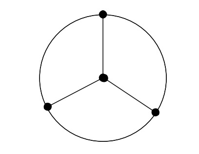
The diameter of a set \(X \subseteq \mathbb{R}^d\) is defined as
18. On the Difficulty of Reducing the Diameter
\(\operatorname{diam}(X):=\sup \{\|\mathbf{x}-\mathbf{y}\|: \mathbf{x}, \mathbf{y} \in X\}\)
Can every set \(X \subset \mathbb{R}^d\) of finite diameter be partitioned into \(d+1\) subsets \(X_1, X_2, \ldots, X_{d+1}\) so that each \(X_i\) has diameter strictly smaller than \(X\)?
NO.
The diameter of a set \(X \subseteq \mathbb{R}^d\) is defined as
18. On the Difficulty of Reducing the Diameter
\(\operatorname{diam}(X):=\sup \{\|\mathbf{x}-\mathbf{y}\|: \mathbf{x}, \mathbf{y} \in X\}\)
Can every set \(X \subset \mathbb{R}^d\) of finite diameter be partitioned into \(d+1\) subsets \(X_1, X_2, \ldots, X_{d+1}\) so that each \(X_i\) has diameter strictly smaller than \(X\)?
Theorem. For every prime \(p\) there exists a point set in \(\mathbb{R}^{n^2}, n=4p\), that has no diameter-reducing partition into fewer than \(1.1^n\) parts.
(pick \(1.1^n > n^2+1\) to see that Theorem \(\implies\) NO.)
The diameter of a set \(X \subseteq \mathbb{R}^d\) is defined as
18. On the Difficulty of Reducing the Diameter
\(\operatorname{diam}(X):=\sup \{\|\mathbf{x}-\mathbf{y}\|: \mathbf{x}, \mathbf{y} \in X\}\)
Theorem. For every prime \(p\) there exists a point set in \(\mathbb{R}^{n^2}, n=4p\), that has no diameter-reducing partition into fewer than \(1.1^n\) parts.
Let \(p\) be a prime number and let \(\mathcal{F}\) be a system of \((2p-1)\) element subsets of an n-element set \(X\) such that no two sets in \(\mathcal{F}\) intersect in precisely \(p-1\) elements.
Then the number of sets in \(\mathcal{F}\) is at most
\(|\mathcal{F}| \leqslant\underbrace{\left(\begin{array}{c}n \\0\end{array}\right)+\left(\begin{array}{c}n \\1\end{array}\right)+\cdots+\left(\begin{array}{c}n \\p-1\end{array}\right)}_{\ell_{n,p}}\)
The diameter of a set \(X \subseteq \mathbb{R}^d\) is defined as
18. On the Difficulty of Reducing the Diameter
\(\operatorname{diam}(X):=\sup \{\|\mathbf{x}-\mathbf{y}\|: \mathbf{x}, \mathbf{y} \in X\}\)
Theorem. For every prime \(p\) there exists a point set in \(\mathbb{R}^{n^2}, n=4p\), that has no diameter-reducing partition into fewer than \(1.1^n\) parts.
Large collection of \(2p-1\) sized-sets
\(\implies\)
a medium sized intersection manifests.
The diameter of a set \(X \subseteq \mathbb{R}^d\) is defined as
18. On the Difficulty of Reducing the Diameter
\(\operatorname{diam}(X):=\sup \{\|\mathbf{x}-\mathbf{y}\|: \mathbf{x}, \mathbf{y} \in X\}\)
Theorem. For every prime \(p\) there exists a point set in \(\mathbb{R}^{n^2}, n=4p\), that has no diameter-reducing partition into fewer than \(1.1^n\) parts.
Let \(\mathcal{X}\) be all the \((2p-1)\) element subsets of an \(n\)-element set \(X\).
If \(\mathcal{X}\) partitioned into fewer than \(t\) parts,
then some part will have more than \(\frac{|\mathcal{X}|}{t}\) elements.
The diameter of a set \(X \subseteq \mathbb{R}^d\) is defined as
18. On the Difficulty of Reducing the Diameter
\(\operatorname{diam}(X):=\sup \{\|\mathbf{x}-\mathbf{y}\|: \mathbf{x}, \mathbf{y} \in X\}\)
Theorem. For every prime \(p\) there exists a point set in \(\mathbb{R}^{n^2}, n=4p\), that has no diameter-reducing partition into fewer than \(1.1^n\) parts.
Let \(\mathcal{X}\) be all the \((2p-1)\) element subsets of an \(n\)-element set \(X\).
If \(\mathcal{X}\) partitioned into fewer than \(1.1^n\) parts,
then some part will have more than \(\frac{|\mathcal{X}|}{1.1^n}\) sets.
If \(\frac{|\mathcal{X}|}{1.1^n} > \ell_{n,p}\), then this part will
also witness a medium-sized intersection.
The diameter of a set \(X \subseteq \mathbb{R}^d\) is defined as
18. On the Difficulty of Reducing the Diameter
\(\operatorname{diam}(X):=\sup \{\|\mathbf{x}-\mathbf{y}\|: \mathbf{x}, \mathbf{y} \in X\}\)
Theorem. For every prime \(p\) there exists a point set in \(\mathbb{R}^{n^2}, n=4p\), that has no diameter-reducing partition into fewer than \(1.1^n\) parts.
Let \(\mathcal{X}\) be all the \((2p-1)\) element subsets of an \(n\)-element set \(X\).
If \(\mathcal{X}\) partitioned into fewer than \(1.1^n\) parts,
then some part will have more than \(\frac{|\mathcal{X}|}{1.1^n}\) sets.
If \(\frac{\binom{n}{2p-1}}{1.1^n} > \ell_{n,p}\), then this part will
also witness a medium-sized intersection.
The diameter of a set \(X \subseteq \mathbb{R}^d\) is defined as
18. On the Difficulty of Reducing the Diameter
\(\operatorname{diam}(X):=\sup \{\|\mathbf{x}-\mathbf{y}\|: \mathbf{x}, \mathbf{y} \in X\}\)
Theorem. For every prime \(p\) there exists a point set in \(\mathbb{R}^{n^2}, n=4p\), that has no diameter-reducing partition into fewer than \(1.1^n\) parts.
Let \(\mathcal{X}\) be all the \((2p-1)\) element subsets of an \(n\)-element set \(X\).
If \(\mathcal{X}\) partitioned into fewer than \(1.1^n\) parts,
then some part will have more than \(\frac{|\mathcal{X}|}{1.1^n}\) sets.
If \({\color{SeaGreen}\frac{\binom{n}{2p-1}}{1.1^n} > \ell_{n,p}}\), then this part will
also witness a medium-sized intersection.
The diameter of a set \(X \subseteq \mathbb{R}^d\) is defined as
18. On the Difficulty of Reducing the Diameter
\(\operatorname{diam}(X):=\sup \{\|\mathbf{x}-\mathbf{y}\|: \mathbf{x}, \mathbf{y} \in X\}\)
Theorem. For every prime \(p\) there exists a point set in \(\mathbb{R}^{n^2}, n=4p\), that has no diameter-reducing partition into fewer than \(1.1^n\) parts.
Let \(\mathcal{X}\) be all the \((2p-1)\) element subsets of an \(n\)-element set \(X\).
If \(\mathcal{X}\) partitioned into fewer than \(1.1^n\) parts,
then some part will have more than \(\frac{|\mathcal{X}|}{1.1^n}\) sets.
If \({\color{SeaGreen}\frac{\binom{n}{2p-1}}{\ell_{n,p}} > 1.1^n}\), then this part will
also witness a medium-sized intersection.
The diameter of a set \(X \subseteq \mathbb{R}^d\) is defined as
18. On the Difficulty of Reducing the Diameter
\(\operatorname{diam}(X):=\sup \{\|\mathbf{x}-\mathbf{y}\|: \mathbf{x}, \mathbf{y} \in X\}\)
Theorem. For every prime \(p\) there exists a point set in \(\mathbb{R}^{n^2}, n=4p\), that has no diameter-reducing partition into fewer than \(1.1^n\) parts.
Let \(\mathcal{X}\) be all the \((2p-1)\) element subsets of an \(4p\)-element set \(X\).
If \(\mathcal{X}\) partitioned into fewer than \(1.1^{4p}\) parts,
then some part will have more than \(\frac{|\mathcal{X}|}{1.1^{4p}}\) sets.
Since \({\color{SeaGreen}\frac{\binom{4p}{2p-1}}{\ell_{4p,p}} > 1.1^{4p}}\), then this part will
also witness a medium-sized intersection.
The diameter of a set \(X \subseteq \mathbb{R}^d\) is defined as
18. On the Difficulty of Reducing the Diameter
\(\operatorname{diam}(X):=\sup \{\|\mathbf{x}-\mathbf{y}\|: \mathbf{x}, \mathbf{y} \in X\}\)
Theorem. For every prime \(p\) there exists a point set in \(\mathbb{R}^{n^2}, n=4p\), that has no diameter-reducing partition into fewer than \(1.1^n\) parts.
\(A \subseteq [n] \Longleftrightarrow \mathbf{c}_A\).
Goal: map sets to points/vectors so that
medium-sized intersections between sets \(A, B\)
\(\Longleftrightarrow\)
large distances between points \(f(A), f(B)\)
\(n = 5; A = \{1,2,5\} \Longleftrightarrow \mathbf{c}_A = (1,1,0,0,1)\)
\(|A \cap B| = p-1 \Longleftrightarrow ||\mathbf{c}_A - \mathbf{c}_B|| = \star\)
The diameter of a set \(X \subseteq \mathbb{R}^d\) is defined as
18. On the Difficulty of Reducing the Diameter
\(\operatorname{diam}(X):=\sup \{\|\mathbf{x}-\mathbf{y}\|: \mathbf{x}, \mathbf{y} \in X\}\)
Theorem. For every prime \(p\) there exists a point set in \(\mathbb{R}^{n^2}, n=4p\), that has no diameter-reducing partition into fewer than \(1.1^n\) parts.
\(A \subseteq [n] \Longleftrightarrow \mathbf{c}_A\).
\(n = 5; A = \{1,2,5\} \Longleftrightarrow \mathbf{c}_A = (1,1,0,0,1)\)
\(|A \cap B| = p-1 \Longleftrightarrow ||\mathbf{c}_A - \mathbf{c}_B|| = \sqrt{2p}\)
Goal: map sets to points/vectors so that
medium-sized intersections between sets \(A, B\)
\(\Longleftrightarrow\)
large distances between points \(f(A), f(B)\)
For any prime \(p\), there exists a collection of points in \(\mathbb{R}^n\)
18. On the Difficulty of Reducing the Diameter
such that if they are partitioned into fewer than \(1.1^n\) parts,
there will be at least one part with two points \(\sqrt{2p}\) apart.
But for this result to be useful, we need it to have diameter \({\color{SeaGreen}= \sqrt{2p}}\).
Clearly the full point set has diameter \(\geqslant \sqrt{2p}\).
Potential problem: original point set has diameter \({\color{IndianRed}> \sqrt{2p}}\).
The diameter of a set \(X \subseteq \mathbb{R}^d\) is defined as
\(\operatorname{diam}(X):=\sup \{\|\mathbf{x}-\mathbf{y}\|: \mathbf{x}, \mathbf{y} \in X\}\)
Theorem. For every prime \(p\) there exists a point set in \(\mathbb{R}^{n^2}, n=4p\), that has no diameter-reducing partition into fewer than \(1.1^n\) parts.
18. On the Difficulty of Reducing the Diameter
The diameter of a set \(X \subseteq \mathbb{R}^d\) is defined as
\(\operatorname{diam}(X):=\sup \{\|\mathbf{x}-\mathbf{y}\|: \mathbf{x}, \mathbf{y} \in X\}\)
Theorem. For every prime \(p\) there exists a point set in \(\mathbb{R}^{n^2}, n=4p\), that has no diameter-reducing partition into fewer than \(1.1^n\) parts.
Goal: map sets to points/vectors so that
medium-sized intersections between sets \(A, B\)
\(\Longleftrightarrow\)
large distances between points \(f(A), f(B)\)
The diameter of a set \(X \subseteq \mathbb{R}^d\) is defined as
18. On the Difficulty of Reducing the Diameter
\(\operatorname{diam}(X):=\sup \{\|\mathbf{x}-\mathbf{y}\|: \mathbf{x}, \mathbf{y} \in X\}\)
Theorem. For every prime \(p\) there exists a point set in \(\mathbb{R}^{n^2}, n=4p\), that has no diameter-reducing partition into fewer than \(1.1^n\) parts.
\(A \subseteq [n] \Longleftrightarrow \mathbf{s}_A\).
\(n = 5; A = \{1,2,5\} \Longleftrightarrow \mathbf{s}_A = (1,1,-1,-1,1)^T\)
\(f(A) = \mathbf{s}_A \cdot \mathbf{s}_A^T \)
The diameter of a set \(X \subseteq \mathbb{R}^d\) is defined as
18. On the Difficulty of Reducing the Diameter
\(\operatorname{diam}(X):=\sup \{\|\mathbf{x}-\mathbf{y}\|: \mathbf{x}, \mathbf{y} \in X\}\)
Theorem. For every prime \(p\) there exists a point set in \(\mathbb{R}^{n^2}, n=4p\), that has no diameter-reducing partition into fewer than \(1.1^n\) parts.
\(A \subseteq [n] \Longleftrightarrow \mathbf{s}_A; A = \{1,2,5\}.\)
\((1,1,-1,-1,1)^T \cdot (1,1,-1,-1,1)\)
\(=\begin{pmatrix}1 & 1 & -1 & -1 & 1 \\1 & 1 & -1 & -1 & 1 \\-1 & -1 & 1 & 1 & -1 \\-1 & -1 & 1 & 1 & -1 \\1 & 1 & -1 & -1 & 1 \\\end{pmatrix}\)
The diameter of a set \(X \subseteq \mathbb{R}^d\) is defined as
18. On the Difficulty of Reducing the Diameter
\(\operatorname{diam}(X):=\sup \{\|\mathbf{x}-\mathbf{y}\|: \mathbf{x}, \mathbf{y} \in X\}\)
Theorem. For every prime \(p\) there exists a point set in \(\mathbb{R}^{n^2}, n=4p\), that has no diameter-reducing partition into fewer than \(1.1^n\) parts.
\(A \subseteq [n] \Longleftrightarrow \mathbf{s}_A; A = \{1,2,5\}.\)
\((1,1,-1,-1,1)^T \cdot (1,1,-1,-1,1)\)
\(= (1, 1, -1, -1, 1, 1, 1, -1, -1, 1, -1, -1, 1, 1, -1, -1, -1, 1, 1, -1, 1, 1, -1, -1, 1 )\)
\(f(A)_{ij} = \begin{cases} +1 & \text{if } i,j \in A \text{ or } i,j \notin A, \\ -1 &\text{otherwise.} \\ \end{cases}\)
The diameter of a set \(X \subseteq \mathbb{R}^d\) is defined as
18. On the Difficulty of Reducing the Diameter
\(\operatorname{diam}(X):=\sup \{\|\mathbf{x}-\mathbf{y}\|: \mathbf{x}, \mathbf{y} \in X\}\)
Theorem. For every prime \(p\) there exists a point set in \(\mathbb{R}^{n^2}, n=4p\), that has no diameter-reducing partition into fewer than \(1.1^n\) parts.
\(A \subseteq [n] \Longleftrightarrow \mathbf{s}_A; A = \{1,2,5\} \Longleftrightarrow (1,1,-1,-1,1)^T\)
\((1, 1, -1, -1, 1, 1, 1, -1, -1, 1, -1, -1, 1, 1, -1, -1, -1, 1, 1, -1, 1, 1, -1, -1, 1 )\)
\(A \subseteq [n] \Longleftrightarrow \mathbf{q}_A = \mathbf{s}_A \mathbf{s}_A^T\)
\((1, -1, 1, -1, 1, -1, 1, -1, 1, -1, 1, -1, 1, -1, 1, -1, 1, -1, 1, -1, 1, -1, 1, -1, 1)\)
\(ij\)
\(ij\)
# of coordinates that clash-and-survive, contributing to the distance:
18. On the Difficulty of Reducing the Diameter
\(\operatorname{diam}(X):=\sup \{\|\mathbf{x}-\mathbf{y}\|: \mathbf{x}, \mathbf{y} \in X\}\)
\(4p\)
\(x\)
\(q\)
\(y\)
(ij) should be: (fully in or fully out of one set) + (split by the other)
...opposite polarities are good for survival; same polarity cancels out.
18. On the Difficulty of Reducing the Diameter
\(\operatorname{diam}(X):=\sup \{\|\mathbf{x}-\mathbf{y}\|: \mathbf{x}, \mathbf{y} \in X\}\)
\(4p\)
\(x\)
\(q\)
\(y\)
(ij) should be: (fully in or fully out of one set) + (split by the other)
\(x \cdot (4p - (x+q+y))\)
# of coordinates that clash-and-survive, contributing to the distance:
18. On the Difficulty of Reducing the Diameter
\(\operatorname{diam}(X):=\sup \{\|\mathbf{x}-\mathbf{y}\|: \mathbf{x}, \mathbf{y} \in X\}\)
\(4p\)
\(x\)
\(q\)
\(y\)
(ij) should be: (fully in or fully out of one set) + (split by the other)
\(y \cdot (4p - (x+q+y))\)
# of coordinates that clash-and-survive, contributing to the distance:
18. On the Difficulty of Reducing the Diameter
\(\operatorname{diam}(X):=\sup \{\|\mathbf{x}-\mathbf{y}\|: \mathbf{x}, \mathbf{y} \in X\}\)
\(4p\)
\(x\)
\(q\)
\(y\)
(ij) should be: (fully in or fully out of one set) + (split by the other)
\(xq\)
# of coordinates that clash-and-survive, contributing to the distance:
18. On the Difficulty of Reducing the Diameter
\(\operatorname{diam}(X):=\sup \{\|\mathbf{x}-\mathbf{y}\|: \mathbf{x}, \mathbf{y} \in X\}\)
\(4p\)
\(x\)
\(q\)
\(y\)
(ij) should be: (fully in or fully out of one set) + (split by the other)
\(yq\)
# of coordinates that clash-and-survive, contributing to the distance:
18. On the Difficulty of Reducing the Diameter
\(\operatorname{diam}(X):=\sup \{\|\mathbf{x}-\mathbf{y}\|: \mathbf{x}, \mathbf{y} \in X\}\)
\(4p\)
\(x\)
\(q\)
\(y\)
(ij) should be: (fully in or fully out of one set) + (split by the other)
\((4px - (x^2+qx+yx))\)
\((4py - (xy+qy+y^2))\)
\(xq\)
\(yq\)
# of coordinates that clash-and-survive, contributing to the distance:
18. On the Difficulty of Reducing the Diameter
\(\operatorname{diam}(X):=\sup \{\|\mathbf{x}-\mathbf{y}\|: \mathbf{x}, \mathbf{y} \in X\}\)
\(4p\)
\(x\)
\(q\)
\(y\)
(ij) should be: (fully in or fully out of one set) + (split by the other)
\((4px - (x^2+yx))\)
\((4py - (xy+y^2))\)
# of coordinates that clash-and-survive, contributing to the distance:
18. On the Difficulty of Reducing the Diameter
\(4p(x+y) - (x+y)^2 = (x+y)(4p - (x + y))\)
\(\operatorname{diam}(X):=\sup \{\|\mathbf{x}-\mathbf{y}\|: \mathbf{x}, \mathbf{y} \in X\}\)
\(4p\)
\(x\)
\(q\)
\(y\)
Disjoint: \(4p(4p-2) - (4p-2)^2 = 8p - 4\)
Medium intersection: \(4p(2p) - (2p)^2 = 4p^2\)
\((p-2)\)-sized intersection: \(4p(2p+2) - (2p+2)^2 = 4p^2 - 4\)
\((p)\)-sized intersection: \(4p(2p-2) - (2p-2)^2 = 4p^2 - 4\)
18. On the Difficulty of Reducing the Diameter
\(4p(x+y) - (x+y)^2 = (x+y)(4p - (x + y))\)
\(\operatorname{diam}(X):=\sup \{\|\mathbf{x}-\mathbf{y}\|: \mathbf{x}, \mathbf{y} \in X\}\)
\(4p\)
\(x\)
\(q\)
\(y\)
\(0 \leqslant \underbrace{(x+y)}_{A \Delta B} \leqslant 4p-2\)
Maximize:
The maximum attained at \(x+y = 2p \equiv \) the sets overlap at \(p-1\) elements.
18. On the Difficulty of Reducing the Diameter
\(4p(x+y) - (x+y)^2 = (x+y)(4p - (x + y))\)
\(\operatorname{diam}(X):=\sup \{\|\mathbf{x}-\mathbf{y}\|: \mathbf{x}, \mathbf{y} \in X\}\)
\(4p\)
\(x\)
\(q\)
\(y\)
Disjoint: \(4p(4p-2) - (4p-2)^2 = 8p - 4\)
Medium intersection: \(4p(2p) - (2p)^2 = 4p^2\)
\((p-2)\)-sized intersection: \(4p(2p+2) - (2p+2)^2 = 4p^2 - 4\)
\((p)\)-sized intersection: \(4p(2p-2) - (2p-2)^2 = 4p^2 - 4\)
The diameter of a set \(X \subseteq \mathbb{R}^d\) is defined as
18. On the Difficulty of Reducing the Diameter
\(\operatorname{diam}(X):=\sup \{\|\mathbf{x}-\mathbf{y}\|: \mathbf{x}, \mathbf{y} \in X\}\)
Theorem. For every prime \(p\) there exists a point set in \(\mathbb{R}^{n^2}, n=4p\), that has no diameter-reducing partition into fewer than \(1.1^n\) parts.
\(A \subseteq [n] \Longleftrightarrow \mathbf{s}_A; A = \{1,2,5\}.\)
\((1,-1,1,-1,1)^T \cdot (1,-1,1,-1,1)\)
\(=\begin{pmatrix}1 & -1 & 1 & -1 & 1 \\-1 & 1 & -1 & 1 & -1 \\1 & -1 & 1 & -1 & 1 \\-1 & 1 & -1 & 1 & -1 \\1 & -1 & 1 & -1 & 1 \\\end{pmatrix}\)
An internet shop was processing \(m\) orders,
each of them asking for various products.
19. The End of Small Coins
{57.14,151.61,85.71,33.33,64.29,40.91}🎁
💍
👘
🥿
🍲
🧶
{64.29,133.33,55.56,151.61,60.00}🏸
💍
☕
🥎
🏏
{60.00,52.73,55.56,233.33,64.29}☕
🍟
🍷
🥎
🍲
Suddenly, all paisa coins were taken out of circulation, and all prices had to be rounded, up or down, to whole rupees.
An internet shop was processing \(m\) orders,
each of them asking for various products.
19. The End of Small Coins
{151.61}💍
{151.61}💍
{151.61}💍
{151.61}💍
{151.61}💍
{151.61}💍
{151.61}💍
{151.61}💍
{151.61}💍
{151.61}💍
{151.61}💍
{151.61}💍
Suddenly, all paisa coins were taken out of circulation, and all prices had to be rounded, up or down, to whole rupees.
An internet shop was processing \(m\) orders,
each of them asking for various products.
19. The End of Small Coins
{57.14,151.61,85.71,33.33,64.29,40.91}🎁
💍
👘
🥿
🍲
🧶
↓14↓61↑29↑67↑71↓91
Suddenly, all paisa coins were taken out of circulation, and all prices had to be rounded, up or down, to whole rupees.
An internet shop was processing \(m\) orders,
each of them asking for various products.
19. The End of Small Coins
If
(a) at most \(t\) pieces of each product have been ordered in total, and
(b) if no order asks for more than one piece of each product,
then:
it is possible to round the prices so that the total price of each order changes by no more than \(t\) rupees.
Suddenly, all paisa coins were taken out of circulation, and all prices had to be rounded, up or down, to whole rupees.
An internet shop was processing \(m\) orders,
each of them asking for various products.
19. The End of Small Coins
{57.14,151.61,85.71,33.33,64.29,40.91}🎁
💍
👘
🥿
🍲
🧶
{64.29,133.33,55.56,151.61,60.00}🏸
💍
☕
🥎
🏏
{60.00,52.73,55.56,233.33,64.29}☕
🍟
🍷
🥎
🍲
Suddenly, all paisa coins were taken out of circulation, and all prices had to be rounded, up or down, to whole rupees.
An internet shop was processing \(m\) orders,
each of them asking for various products.
19. The End of Small Coins
If
(a) at most \(t\) pieces of each product have been ordered in total, and
(b) if no order asks for more than one piece of each product,
then:
it is possible to round the prices so that the total price of each order changes by no more than \(t\) rupees.
Suddenly, all paisa coins were taken out of circulation, and all prices had to be rounded, up or down, to whole rupees.
An internet shop was processing \(m\) orders,
each of them asking for various products.
19. The End of Small Coins
Global pool of items: \([n]\)
Orders: \(\{S_1, \ldots, S_m\},\) where \(S_i \subseteq [n]\).
If no \(j\) is in more than \(t\) sets,
then there are numbers \(z_1, z_2, \ldots, z_n \in\{0,1\}\) such that
\(\left|\sum_{j \in S_i} c_j-\sum_{j \in S_i} z_j\right| \leq t, \quad \text { for every } i=1,2, \ldots, m\)
Suddenly, all paisa coins were taken out of circulation, and all prices had to be rounded, up or down, to whole rupees.
19. The End of Small Coins
Call an order nice if it has fewer than \(t\) products. (why?)
Call an order large if it has more than \(t\) products.
# products 🤝 # large orders
at most \(t\) edges
more than \(t\) edges
If (a) at most \(t\) pieces of each product have been ordered in total, and
(b) if no order asks for more than one piece of each product,
then: it is possible to round the prices so that the total price of each order changes by no more than \(t\) rupees.
19. The End of Small Coins
Call an order nice if it has fewer than \(t\) products. (why?)
Call an order large if it has more than \(t\) products.
at most \(t\) edges
more than \(t\) edges
\(t \cdot\) (# products) \(\geqslant\) # edges \(>\) (# large orders) \(\cdot t\)
If (a) at most \(t\) pieces of each product have been ordered in total, and
(b) if no order asks for more than one piece of each product,
then: it is possible to round the prices so that the total price of each order changes by no more than \(t\) rupees.
19. The End of Small Coins
Call an order nice if it has fewer than \(t\) products. (why?)
Call an order large if it has more than \(t\) products.
at most \(t\) edges
more than \(t\) edges
(# products) \(\geqslant\) # edges \(>\) (# large orders)
If (a) at most \(t\) pieces of each product have been ordered in total, and
(b) if no order asks for more than one piece of each product,
then: it is possible to round the prices so that the total price of each order changes by no more than \(t\) rupees.
19. The End of Small Coins
Call an order nice if it has fewer than \(t\) products. (why?)
Call an order large if it has more than \(t\) products.
at most \(t\) edges
more than \(t\) edges
(# products) \(>\) (# large orders)
If (a) at most \(t\) pieces of each product have been ordered in total, and
(b) if no order asks for more than one piece of each product,
then: it is possible to round the prices so that the total price of each order changes by no more than \(t\) rupees.
19. The End of Small Coins
Introduce variables:
\(x_1 = {\color{IndianRed}c_1}, \ldots, x_n = {\color{IndianRed}c_n}\)
If (a) at most \(t\) pieces of each product have been ordered in total, and
(b) if no order asks for more than one piece of each product,
then: it is possible to round the prices so that the total price of each order changes by no more than \(t\) rupees.
\(x_i\) will be the final price of product \(i\).
To begin with, \(x_i\) is initialized to the original price of product \(i\).
It will eventually evolve to either \(0\) or \(1\),
in way that is compatible with our overarching goal.
Interim stages: \(x_i\) is floating if it's value is in (0,1); and final otherwise.
19. The End of Small Coins
Introduce variables:
\(x_1 = {\color{IndianRed}c_1}, \ldots, x_n = {\color{IndianRed}c_n}\)
If (a) at most \(t\) pieces of each product have been ordered in total, and
(b) if no order asks for more than one piece of each product,
then: it is possible to round the prices so that the total price of each order changes by no more than \(t\) rupees.
\(x_i\) will be the final price of product \(i\).
Call a set \(S_i\) dangerous if it has more than \(t\) floating variables.
Maintain: \({\color{IndianRed}\sum_{i \in S_i} x_i = \sum_{i \in S_i} c_i}\)
for all dangerous sets.
Interpret this as a system of equations where
floating variables are unknowns and final variables are constants.
19. The End of Small Coins
If (a) at most \(t\) pieces of each product have been ordered in total, and
(b) if no order asks for more than one piece of each product,
then: it is possible to round the prices so that the total price of each order changes by no more than \(t\) rupees.
#unknowns 🤝 #constraints
Call a set \(S_i\) dangerous if it has more than \(t\) floating variables.
Maintain: \({\color{IndianRed}\sum_{j \in S_i} x_j = \sum_{j \in S_i} c_j}\)
for all dangerous sets.
Interpret this as a system of equations where
floating variables are unknowns and final variables are constants.
19. The End of Small Coins
If (a) at most \(t\) pieces of each product have been ordered in total, and
(b) if no order asks for more than one piece of each product,
then: it is possible to round the prices so that the total price of each order changes by no more than \(t\) rupees.
#unknowns \(>\) #constraints
Call a set \(S_i\) dangerous if it has more than \(t\) floating variables.
Maintain: \({\color{IndianRed}\sum_{i \in S_i} x_i = \sum_{i \in S_i} c_i}\)
for all dangerous sets.
Interpret this as a system of equations where
floating variables are unknowns and final variables are constants.
19. The End of Small Coins
If (a) at most \(t\) pieces of each product have been ordered in total, and
(b) if no order asks for more than one piece of each product,
then: it is possible to round the prices so that the total price of each order changes by no more than \(t\) rupees.
underdetermined system with at least one solution
Call a set \(S_i\) dangerous if it has more than \(t\) floating variables.
Maintain: \({\color{IndianRed}\sum_{i \in S_i} x_i = \sum_{i \in S_i} c_i}\)
for all dangerous sets.
Interpret this as a system of equations where
floating variables are unknowns and final variables are constants.
19. The End of Small Coins
If (a) at most \(t\) pieces of each product have been ordered in total, and
(b) if no order asks for more than one piece of each product,
then: it is possible to round the prices so that the total price of each order changes by no more than \(t\) rupees.
The solution space has dimension \(\geqslant 1\).
Call a set \(S_i\) dangerous if it has more than \(t\) floating variables.
Maintain: \({\color{IndianRed}\sum_{i \in S_i} x_i = \sum_{i \in S_i} c_i}\)
for all dangerous sets.
Interpret this as a system of equations where
floating variables are unknowns and final variables are constants.
underdetermined system with at least one solution
\(\underbrace{~~~~~~~~~~~~~~~~~~~~~~~~~~~~~~~~~~~~~~~~~~~~~}\)
\(\underbrace{~~~~~~~~~~~~~~~~~~~~~~~~~~~~~~~~~}\)
Interior point of \([0,1]^{|F|}\).
19. The End of Small Coins
If (a) at most \(t\) pieces of each product have been ordered in total, and
(b) if no order asks for more than one piece of each product,
then: it is possible to round the prices so that the total price of each order changes by no more than \(t\) rupees.
The solution space has dimension \(\geqslant 1\).
Call a set \(S_i\) dangerous if it has more than \(t\) floating variables.
Maintain: \({\color{IndianRed}\sum_{i \in S_i} x_i = \sum_{i \in S_i} c_i}\)
for all dangerous sets.
There exists a solution where at least one variable is set to \(\{0,1\}\).
underdetermined system with at least one solution
\(\underbrace{~~~~~~~~~~~~~~~~~~~~~~~~~~~~~~~~~~~~~~~~~~~~~}\)
\(\underbrace{~~~~~~~~~~~~~~~~~~~~~~~~~~~~~~~~~}\)
Interior point of \([0,1]^{|F|}\).
Rinse and repeat.
20. Walking in the Yard
👾
🐍
🔥
2/3
2/3
1/3
1
2/3
1/3
1
1/3
1
1
1
20. Walking in the Yard
👾
🐍
🔥
2/3
1/3
-1/3
-2/3
0
-1
-1/3
1
0
Four green (left)
segments of length
one each
One red (right)
segment of length one,
three of length 2/3,
three of length 1/3.
20. Walking in the Yard
🛍️
🛍️
🛍️
🛍️
🛍️
🛍️
🛍️
🛍️
🚶♀️
\(\underbrace{~~~~~~~~~~~~~~~~~~~~~~~~~~~~~~~~~}\)
\(2\)
\(\underbrace{~~~~~~~~~~~~~~~~~}\)
\(1\)
20. Walking in the Yard
🛍️
🛍️
🛍️
🛍️
🛍️
🛍️
🛍️
🛍️
🚶♀️
20. Walking in the Yard
🛍️
🛍️
🛍️
🛍️
🛍️
🛍️
🛍️
🛍️
🚶♀️
20. Walking in the Yard
🛍️
🛍️
🛍️
🛍️
🛍️
🛍️
🛍️
🛍️
🚶♀️
20. Walking in the Yard
Let \(M\) be an arbitrary set of \(n\) vectors in \(\mathbb{R}^d\) such that \(\|\mathbf{v}\| \leqslant 1\) for every \(\mathbf{v} \in M\).
Then it is possible to arrange all vectors of \(M\) into a sequence
\(\left(\mathbf{v}_1, \mathbf{v}_2, \ldots, \mathbf{v}_n\right)\)
in such a way that \(\left\|\mathbf{v}_1+\mathbf{v}_2+\cdots+\mathbf{v}_k\right\| \leqslant d\) for every \(k=1,2, \ldots, n\).
Lemma. Let \(A \mathbf{x}=\mathbf{b}\) be a system of \(m\) linear equations in \(n \geq m\) unknowns,
and let us suppose that it has a solution \(\mathbf{x}_0 \in[0,1]^n\).
Then there is a solution \(\tilde{\mathbf{x}} \in[0,1]^n\) in which at least \(n-m\) components are 0 's or 1 's.
20. Walking in the Yard
🚶♀️
What if there are only \(d+1\) vectors?
20. Walking in the Yard
A set \(K=\left\{\mathbf{w}_1, \mathbf{w}_2, \ldots, \mathbf{w}_k\right\}\) of \(k \geqslant d\) vectors in \(\mathbb{R}^d\), each of length at most 1,
is called good
if there exist coefficients \(\alpha_1, \ldots, \alpha_k\) satisfying
\(\alpha_i \in[0,1], \quad i=1,2, \ldots, k\)
\(\alpha_1 \mathbf{w}_1+\alpha_2 \mathbf{w}_2+\cdots+\alpha_k \mathbf{w}_k=\mathbf{0}\)
\(\alpha_1+\alpha_2+\cdots+\alpha_k=k-d\)
20. Walking in the Yard
Wishful Thinking. If \(K=\left\{\mathbf{w}_1, \mathbf{w}_2, \ldots, \mathbf{w}_k\right\}\) is a \(d\)-bounded set of \(k>d\) vectors,
then there is some \(i\) such that
\(K \backslash\left\{\mathbf{w}_i\right\}\) is a \(d\)-bounded set of \(k-1\) vectors.
Definition. \(K=\left\{\mathbf{w}_1, \mathbf{w}_2, \ldots, \mathbf{w}_k\right\}\) is \(d\)-bounded if \(\left\|\mathbf{w}_1+\mathbf{w}_2+\cdots+\mathbf{w}_k\right\| \leq d\).
Walking Algorithm \(d=2\)
\(K_0 := \left\{\mathbf{w}_1, \mathbf{w}_2, \mathbf{w}_3, \mathbf{w}_4, \mathbf{w}_5\right\}\) - \(2\) bounded, apply Claim, say Claim returns \(\mathbf{w}_3\).
\(K_1 := \left\{\mathbf{w}_1, \mathbf{w}_2, \mathbf{w}_4, \mathbf{w}_5\right\}\) - \(2\) bounded, apply Claim, say Claim returns \(\mathbf{w}_1\).
\(K_2 := \left\{\mathbf{w}_2, \mathbf{w}_4, \mathbf{w}_5\right\}\) - \(2\) bounded, apply Claim, say Claim returns \(\mathbf{w}_4\).
Safe walk: \(\mathbf{w}_2 \rightarrow \mathbf{w}_5 \rightarrow \mathbf{w}_4 \rightarrow \mathbf{w}_1 \rightarrow \mathbf{w}_3\)
20. Walking in the Yard
A set \(K=\left\{\mathbf{w}_1, \mathbf{w}_2, \ldots, \mathbf{w}_k\right\}\) of \(k \geqslant d\) vectors in \(\mathbb{R}^d\), each of length at most 1,
is called good if there exist coefficients \(\alpha_1, \ldots, \alpha_k\) satisfying
\(\alpha_i \in[0,1], \quad i=1,2, \ldots, k\)
\(\alpha_1 \mathbf{w}_1+\alpha_2 \mathbf{w}_2+\cdots+\alpha_k \mathbf{w}_k=\mathbf{0}\)
\(\alpha_1+\alpha_2+\cdots+\alpha_k=k-d\)
Claim. If \(K=\left\{\mathbf{w}_1, \mathbf{w}_2, \ldots, \mathbf{w}_k\right\}\) is good, then \(\left\|\mathbf{w}_1+\mathbf{w}_2+\cdots+\mathbf{w}_k\right\| \leqslant d\).
Claim. If \(K=\left\{\mathbf{w}_1, \mathbf{w}_2, \ldots, \mathbf{w}_k\right\}\) is a good set of \(k>d\) vectors,
then there is some \(i\) such that \(K \backslash\left\{\mathbf{w}_i\right\}\) is a good set of \(k-1\) vectors.
20. Walking in the Yard
A set \(K=\left\{\mathbf{w}_1, \mathbf{w}_2, \ldots, \mathbf{w}_k\right\}\) of \(k \geqslant d\) vectors in \(\mathbb{R}^d\), each of length at most 1,
is called good if there exist coefficients \(\alpha_1, \ldots, \alpha_k\) satisfying
\(\alpha_i \in[0,1], \quad i=1,2, \ldots, k\)
\(\alpha_1 \mathbf{w}_1+\alpha_2 \mathbf{w}_2+\cdots+\alpha_k \mathbf{w}_k=\mathbf{0}\)
\(\alpha_1+\alpha_2+\cdots+\alpha_k=k-d\)
Claim. If \(K=\left\{\mathbf{w}_1, \mathbf{w}_2, \ldots, \mathbf{w}_k\right\}\) is a good set of \(k>d\) vectors,
then there is some \(i\) such that \(K \backslash\left\{\mathbf{w}_i\right\}\) is a good set of \(k-1\) vectors.
\(\begin{aligned} x_1 \mathbf{w}_1+x_2 \mathbf{w}_2+\cdots+x_k \mathbf{w}_k & =\mathbf{0} \\ x_1+x_2+\cdots+x_k & =k-d-1 .\end{aligned}\)
20. Walking in the Yard
A set \(K=\left\{\mathbf{w}_1, \mathbf{w}_2, \ldots, \mathbf{w}_k\right\}\) of \(k \geqslant d\) vectors in \(\mathbb{R}^d\), each of length at most 1,
is called good if there exist coefficients \(\alpha_1, \ldots, \alpha_k\) satisfying
\(\alpha_i \in[0,1], \quad i=1,2, \ldots, k\)
\(\alpha_1 \mathbf{w}_1+\alpha_2 \mathbf{w}_2+\cdots+\alpha_k \mathbf{w}_k=\mathbf{0}\)
\(\alpha_1+\alpha_2+\cdots+\alpha_k=k-d\)
#variables 🤝 #equations
Claim. If \(K=\left\{\mathbf{w}_1, \mathbf{w}_2, \ldots, \mathbf{w}_k\right\}\) is a good set of \(k>d\) vectors,
then there is some \(i\) such that \(K \backslash\left\{\mathbf{w}_i\right\}\) is a good set of \(k-1\) vectors.
\(\begin{aligned} x_1 \mathbf{w}_1+x_2 \mathbf{w}_2+\cdots+x_k \mathbf{w}_k & =\mathbf{0} \\ x_1+x_2+\cdots+x_k & =k-d-1 .\end{aligned}\)
20. Walking in the Yard
A set \(K=\left\{\mathbf{w}_1, \mathbf{w}_2, \ldots, \mathbf{w}_k\right\}\) of \(k \geqslant d\) vectors in \(\mathbb{R}^d\), each of length at most 1,
is called good if there exist coefficients \(\alpha_1, \ldots, \alpha_k\) satisfying
\(\alpha_i \in[0,1], \quad i=1,2, \ldots, k\)
\(\alpha_1 \mathbf{w}_1+\alpha_2 \mathbf{w}_2+\cdots+\alpha_k \mathbf{w}_k=\mathbf{0}\)
\(\alpha_1+\alpha_2+\cdots+\alpha_k=k-d\)
\(k \geqslant d+1\)
\(\begin{aligned} x_1 \mathbf{w}_1+x_2 \mathbf{w}_2+\cdots+x_k \mathbf{w}_k & =\mathbf{0} \\ x_1+x_2+\cdots+x_k & =k-d-1 .\end{aligned}\)
Claim. If \(K=\left\{\mathbf{w}_1, \mathbf{w}_2, \ldots, \mathbf{w}_k\right\}\) is a good set of \(k>d\) vectors,
then there is some \(i\) such that \(K \backslash\left\{\mathbf{w}_i\right\}\) is a good set of \(k-1\) vectors.
20. Walking in the Yard
A set \(K=\left\{\mathbf{w}_1, \mathbf{w}_2, \ldots, \mathbf{w}_k\right\}\) of \(k \geqslant d\) vectors in \(\mathbb{R}^d\), each of length at most 1,
is called good if there exist coefficients \(\alpha_1, \ldots, \alpha_k\) satisfying
\(\alpha_i \in[0,1], \quad i=1,2, \ldots, k\)
\(\alpha_1 \mathbf{w}_1+\alpha_2 \mathbf{w}_2+\cdots+\alpha_k \mathbf{w}_k=\mathbf{0}\)
\(\alpha_1+\alpha_2+\cdots+\alpha_k=k-d\)
Solvable?
\(\begin{aligned} x_1 \mathbf{w}_1+x_2 \mathbf{w}_2+\cdots+x_k \mathbf{w}_k & =\mathbf{0} \\ x_1+x_2+\cdots+x_k & =k-d-1 .\end{aligned}\)
Claim. If \(K=\left\{\mathbf{w}_1, \mathbf{w}_2, \ldots, \mathbf{w}_k\right\}\) is a good set of \(k>d\) vectors,
then there is some \(i\) such that \(K \backslash\left\{\mathbf{w}_i\right\}\) is a good set of \(k-1\) vectors.
20. Walking in the Yard
A set \(K=\left\{\mathbf{w}_1, \mathbf{w}_2, \ldots, \mathbf{w}_k\right\}\) of \(k \geqslant d\) vectors in \(\mathbb{R}^d\), each of length at most 1,
is called good if there exist coefficients \(\alpha_1, \ldots, \alpha_k\) satisfying
\(\alpha_i \in[0,1], \quad i=1,2, \ldots, k\)
\(\alpha_1 \mathbf{w}_1+\alpha_2 \mathbf{w}_2+\cdots+\alpha_k \mathbf{w}_k=\mathbf{0}\)
\(\alpha_1+\alpha_2+\cdots+\alpha_k=k-d\)
\(x_i := \frac{k-d-1}{k-d} \alpha_i\)
\(\begin{aligned} x_1 \mathbf{w}_1+x_2 \mathbf{w}_2+\cdots+x_k \mathbf{w}_k & =\mathbf{0} \\ x_1+x_2+\cdots+x_k & =k-d-1 .\end{aligned}\)
Claim. If \(K=\left\{\mathbf{w}_1, \mathbf{w}_2, \ldots, \mathbf{w}_k\right\}\) is a good set of \(k>d\) vectors,
then there is some \(i\) such that \(K \backslash\left\{\mathbf{w}_i\right\}\) is a good set of \(k-1\) vectors.
20. Walking in the Yard
A set \(K=\left\{\mathbf{w}_1, \mathbf{w}_2, \ldots, \mathbf{w}_k\right\}\) of \(k \geqslant d\) vectors in \(\mathbb{R}^d\), each of length at most 1,
is called good if there exist coefficients \(\alpha_1, \ldots, \alpha_k\) satisfying
\(\alpha_i \in[0,1], \quad i=1,2, \ldots, k\)
\(\alpha_1 \mathbf{w}_1+\alpha_2 \mathbf{w}_2+\cdots+\alpha_k \mathbf{w}_k=\mathbf{0}\)
\(\alpha_1+\alpha_2+\cdots+\alpha_k=k-d\)
There is also a solution \(\tilde{\mathbf{x}} \in[0,1]^k\) with at least \(k-d-1\) components equal to 0 or 1.
\(\begin{aligned} x_1 \mathbf{w}_1+x_2 \mathbf{w}_2+\cdots+x_k \mathbf{w}_k & =\mathbf{0} \\ x_1+x_2+\cdots+x_k & =k-d-1 .\end{aligned}\)
Claim. If \(K=\left\{\mathbf{w}_1, \mathbf{w}_2, \ldots, \mathbf{w}_k\right\}\) is a good set of \(k>d\) vectors,
then there is some \(i\) such that \(K \backslash\left\{\mathbf{w}_i\right\}\) is a good set of \(k-1\) vectors.
At least one of these components must be zero.
20. Walking in the Yard
A set \(K=\left\{\mathbf{w}_1, \mathbf{w}_2, \ldots, \mathbf{w}_k\right\}\) of \(k \geqslant d\) vectors in \(\mathbb{R}^d\), each of length at most 1,
is called good if there exist coefficients \(\alpha_1, \ldots, \alpha_k\) satisfying
\(\alpha_i \in[0,1], \quad i=1,2, \ldots, k\)
\(\alpha_1 \mathbf{w}_1+\alpha_2 \mathbf{w}_2+\cdots+\alpha_k \mathbf{w}_k=\mathbf{0}\)
\(\alpha_1+\alpha_2+\cdots+\alpha_k=k-d\)
There is also a solution \(\tilde{\mathbf{x}} \in[0,1]^k\) with at least \(k-d-1\) components equal to 0 or 1.
\(\begin{aligned} x_1 \mathbf{w}_1+x_2 \mathbf{w}_2+\cdots+x_k \mathbf{w}_k & =\mathbf{0} \\ x_1+x_2+\cdots+x_k & =k-d-1 .\end{aligned}\)
Claim. If \(K=\left\{\mathbf{w}_1, \mathbf{w}_2, \ldots, \mathbf{w}_k\right\}\) is a good set of \(k>d\) vectors,
then there is some \(i\) such that \(K \backslash\left\{\mathbf{w}_i\right\}\) is a good set of \(k-1\) vectors.
\(\tilde{\mathbf{x_i}} = 0\)
20. Walking in the Yard
A set \(K=\left\{\mathbf{w}_1, \mathbf{w}_2, \ldots, \mathbf{w}_k\right\}\) of \(k \geqslant d\) vectors in \(\mathbb{R}^d\), each of length at most 1,
is called good if there exist coefficients \(\alpha_1, \ldots, \alpha_k\) satisfying
\(\alpha_i \in[0,1], \quad i=1,2, \ldots, k\)
\(\alpha_1 \mathbf{w}_1+\alpha_2 \mathbf{w}_2+\cdots+\alpha_k \mathbf{w}_k=\mathbf{0}\)
\(\alpha_1+\alpha_2+\cdots+\alpha_k=k-d\)
Claim. If \(K=\left\{\mathbf{w}_1, \mathbf{w}_2, \ldots, \mathbf{w}_k\right\}\) is good, then \(\left\|\mathbf{w}_1+\mathbf{w}_2+\cdots+\mathbf{w}_k\right\| \leqslant d\).
\(\begin{aligned}\left\|\sum_{i=1}^k \mathbf{w}_i\right\| & =\left\|\sum_{i=1}^k \mathbf{w}_i-\sum_{i=1}^k \alpha_i \mathbf{w}_i\right\| \\ & \leqslant \sum_{i=1}^k\left\|\left(1-\alpha_i\right) \mathbf{w}_i\right\|=\sum_{i=1}^k\left(1-\alpha_i\right)\left\|\mathbf{w}_i\right\| \\ & \leqslant \sum_{i=1}^k\left(1-\alpha_i\right)=d\end{aligned}\)
21. Counting Spanning Trees
The matrix-tree theorem
21. Counting Spanning Trees
A path is a sequence of edges
\(e_1, \ldots, e_{n-1}\)
such that there exists a sequence of vertices
\(v_1, \ldots, v_n\)
for which \(e_i = (v_i, v_{i+1})\)
for all \(1 \leqslant i \leqslant n-1\),
where all vertices are distinct.
Definitions
21. Counting Spanning Trees
Definitions
A cycle is a sequence of edges
\(e_1, \ldots, e_{n-1}\)
such that there exists a sequence of vertices
\(v_1, \ldots, v_n\)
for which \(e_i = (v_i, v_{i+1})\)
for all \(1 \leqslant i \leqslant n-1\),
where all vertices are distinct except \(v_n = v_1\).
21. Counting Spanning Trees
Definitions
A spanning tree is a subset of edges
\(e_1, \ldots, e_{n-1}\)
such that the subgraph induced by just these edges is
(a) connected
(b) acyclic
In other words, a spanning tree is
a minimally connected subgraph.
21. Counting Spanning Trees
Examples
21. Counting Spanning Trees
not a spanning tree because the
graph induced by the edges is not connected
Examples
21. Counting Spanning Trees
Examples
not a spanning tree because the
graph induced by the edges has a cycle
21. Counting Spanning Trees
Examples
#edges in a spanning tree = #vertices - 1
21. Counting Spanning Trees
#edges in a spanning tree = #vertices - 1
Claim: every tree on at least two vertices has at least two leaves (i.e, vertices of degree one).
Proof (idea). Let \(P\) be a maximal path. Let the endpoints of \(P\) be \(u\) and \(v\).
Note that \(u\) and \(v\) have degree at least one, since they have a neighbor on the path.
Further, they have degree at most one because they cannot have any additional neighbors on the path (this would lead to cycles), or off it (this would contradict the maximality of \(P\)).
21. Counting Spanning Trees
#edges in a spanning tree = #vertices - 1
Induction hypothesis: every tree on n vertices has \(n-1\) edges.
Induction Step (idea).
Let \(T\) be a tree on \(n+1\) vertices,
and let \(v\) be a leaf in \(T\).
Apply the induction hypothesis to \(T \setminus \{v\}\) to see that \(T\) has \(n\) edges.
(Note that \(T \setminus \{v\}\) is a tree.)
21. Counting Spanning Trees
The Laplacian of a Graph
Let \(L\) be the Laplace matrix of \(G\), i.e.,
the \(n \times n\) matrix whose entry \(\ell_{i j}\) is given by:
\(\ell_{i j}:= \begin{cases}\operatorname{deg}(i) & \text { if } i=j \\ -1 & \text { if }\{i, j\} \in E(G) \\ 0 & \text { otherwise }\end{cases}\)
21. Counting Spanning Trees

The Laplacian of a Graph

21. Counting Spanning Trees
Consider the Laplacian of \(G\)...
...with one vertex knocked out.
21. Counting Spanning Trees
Let \(L^{-}\) be the \((n-1) \times(n-1)\) matrix obtained
by deleting the last row and last column of \(L\).
Then:
\({\color{IndianRed}\kappa(G)=\operatorname{det}\left(L^{-}\right).}\)
The matrix-tree theorem
21. Counting Spanning Trees
Consider the Laplacian of \(G\) with one vertex knocked out.
What are the terms of \(\operatorname{det}(L^{-})\)?
How can we interpret them in \(G\)?
21. Counting Spanning Trees
\(\operatorname{det}\left(L^{-}\right)=\sum_\pi \operatorname{sgn}(\pi) \prod_{i=1}^{n-1} \ell_{i, \pi(i)}\)
The product form of the Determinant
21. Counting Spanning Trees

21. Counting Spanning Trees

21. Counting Spanning Trees

21. Counting Spanning Trees

21. Counting Spanning Trees
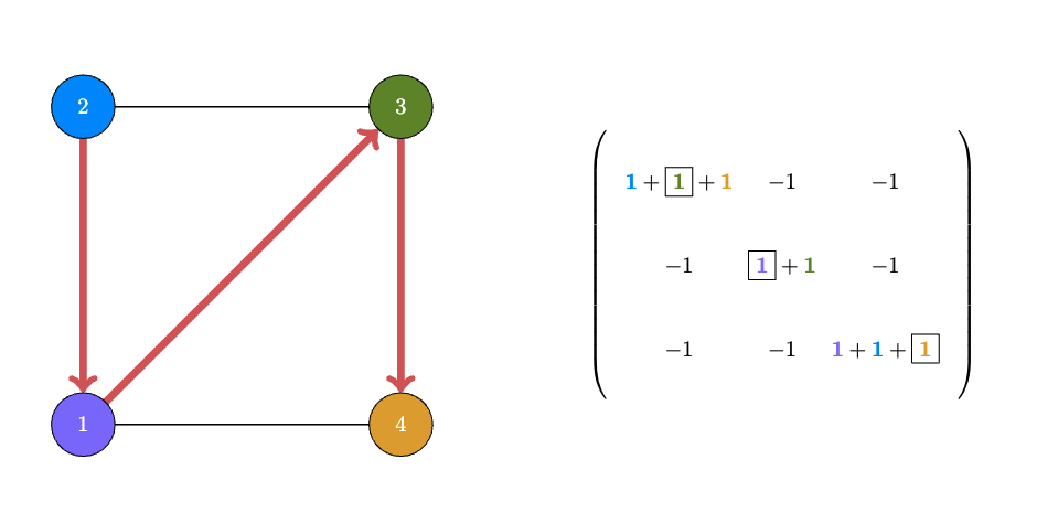
21. Counting Spanning Trees

21. Counting Spanning Trees

21. Counting Spanning Trees

21. Counting Spanning Trees

21. Counting Spanning Trees

21. Counting Spanning Trees

21. Counting Spanning Trees

21. Counting Spanning Trees
If there is a circled -1 in row \(i\) and column \(j\),
make a negative directed edge from \(i\) to \(j\).
If the \(k^{th}\) 1 in the diagonal entry \(\ell_{ii}\) is circled,
make a positive directed edge from \(i\) to the \(k^{th}\) smallest* neighbor of \(i\) in \(G\).
(The vertices of \(G\) are numbered, so we can talk about the \(k^{th}\) smallest neighbor.)
21. Counting Spanning Trees

21. Counting Spanning Trees

21. Counting Spanning Trees

21. Counting Spanning Trees

21. Counting Spanning Trees

21. Counting Spanning Trees

21. Counting Spanning Trees

21. Counting Spanning Trees

21. Counting Spanning Trees
If \(i \rightarrow j\) is a directed edge, then \(\{i, j\}\) is an edge of \(G\).
In the directed graph corresponding to at term in the superexpansion...
If a vertex \(i\) has a negative incoming edge, then the outgoing edge is also negative.
Every vertex, with the exception of \(n\), has exactly one outgoing edge, while \(n\) has no outgoing edge.
All edges incoming onto \(n\) are positive.
No vertex has more than one negative incoming edge.
This is because two negative incoming edges \(j \rightarrow i\) and \(k \rightarrow i\)
would mean two circled entries \(\ell_{j i}\) and \(\ell_{k i}\) in the \(i^{th}\) column.
Indeed, a negative incoming edge \(j \rightarrow i\) means that the off-diagonal entry \(\ell_{ji}\) is circled, and hence none of the 1's in the diagonal entry \(\ell_{i i}\) may be circled (which would be the only way of getting a positive outgoing edge from \(i\)).
21. Counting Spanning Trees

21. Counting Spanning Trees

\(\operatorname{sgn}(D)=\operatorname{sgn}\left(\pi_D\right)(-1)^m\)
21. Counting Spanning Trees
\(\operatorname{sgn}(\sigma) = (−1)^{m}\),
where m is the number of transpositions in the decomposition of \(\sigma\).
1
2
4
7
5
6
21. Counting Spanning Trees
\(\operatorname{sgn}(\sigma) = (−1)^{m}\),
where m is the number of transpositions in the decomposition of \(\sigma\).
1
2
4
7
5
6
\(\operatorname{sgn}(\bar{D})=\operatorname{sgn}\left(\pi_{\bar{D}}\right)(-1)^{m+s}=(-1)^{s-1} \operatorname{sgn}\left(\pi_D\right)(-1)^{m+s}=-\operatorname{sgn}(D)\)
22. In How Many Ways Can
a Man Tile a Board?
Kasteleyn signing
22. In How Many Ways Can
a Man Tile a Board?
22. In How Many Ways Can
a Man Tile a Board?

Tiling
Matching
22. In How Many Ways Can
a Man Tile a Board?
22. In How Many Ways Can
a Man Tile a Board?
Bipartite Graphs: A graph whose vertices can be colored in such a way that no two vertices of the same color are adjacent.
\(\begin{pmatrix}\small{1} & \small{0} & \small{1} & \small{0} & \small{0} \\ \small{0} & \small{1} & \small{0} & \small{1} & \small{0} \\ \small{1} & \small{0} & \small{0} & \small{0} & \small{1} \\ \small{0} & \small{1} & \small{0} & \small{0} & \small{0} \\ \small{0} & \small{0} & \small{1} & \small{0} & \small{1} \\ \end{pmatrix}\)
22. In How Many Ways Can
a Man Tile a Board?
\(b_{i j}:= \begin{cases}1 & \text { if }\left\{u_i, v_j\right\} \in E(G) \\ 0 & \text { otherwise }\end{cases}\)
\(\begin{pmatrix}\small{1} & \small{0} & \small{1} & \small{0} & \small{0} \\ \small{0} & \small{1} & \small{0} & \small{1} & \small{0} \\ \small{1} & \small{0} & \small{0} & \small{0} & \small{1} \\ \small{0} & \small{1} & \small{0} & \small{0} & \small{0} \\ \small{0} & \small{0} & \small{1} & \small{0} & \small{1} \\ \end{pmatrix}\)
22. In How Many Ways Can
a Man Tile a Board?
matchings \(\longleftrightarrow\) permutation entries
\(\begin{pmatrix}{\color{SeaGreen}{\small{1}}} & \small{0} & \small{1} & \small{0} & \small{0} \\ \small{0} & \small{1} & \small{0} & {\color{SeaGreen}{\small{1}}} & \small{0} \\ \small{1} & \small{0} & \small{0} & \small{0} & {\color{SeaGreen}{\small{1}}} \\ \small{0} & {\color{SeaGreen}{\small{1}}} & \small{0} & \small{0} & \small{0} \\ \small{0} & \small{0} & {\color{SeaGreen}{\small{1}}} & \small{0} & \small{1} \\\end{pmatrix}\)
22. In How Many Ways Can
a Man Tile a Board?
\(\begin{pmatrix}{\color{SeaGreen}{\small{1}}} & \small{0} & \small{1} & \small{0} & \small{0} \\ \small{0} & \small{1} & \small{0} & {\color{SeaGreen}{\small{1}}} & \small{0} \\ \small{1} & \small{0} & \small{0} & \small{0} & {\color{SeaGreen}{\small{1}}} \\ \small{0} & {\color{SeaGreen}{\small{1}}} & \small{0} & \small{0} & \small{0} \\ \small{0} & \small{0} & {\color{SeaGreen}{\small{1}}} & \small{0} & \small{1} \\\end{pmatrix}\)
\(\operatorname{per}(B_G) := \sum_{\pi \in S_n} b_{1, \pi(1)} b_{2, \pi(2)} \cdots b_{n, \pi(n)}\)
22. In How Many Ways Can
a Man Tile a Board?
\(\operatorname{per}(B_G) := \sum_{\pi \in S_n} b_{1, \pi(1)} b_{2, \pi(2)} \cdots b_{n, \pi(n)}\)
22. In How Many Ways Can
a Man Tile a Board?
\(\operatorname{per}(B_G) := \sum_{\pi \in S_n} b_{1, \pi(1)} b_{2, \pi(2)} \cdots b_{n, \pi(n)}\)
22. In How Many Ways Can
a Man Tile a Board?
\(\operatorname{per}(B_G) := \sum_{\pi \in S_n} b_{1, \pi(1)} b_{2, \pi(2)} \cdots b_{n, \pi(n)}\)
22. In How Many Ways Can
a Man Tile a Board?
\(\operatorname{per}(B_G) := \sum_{\pi \in S_n} b_{1, \pi(1)} b_{2, \pi(2)} \cdots b_{n, \pi(n)}\)
\(\begin{pmatrix}\small{1} & \small{0} & \small{1} & \small{0} & \small{0} \\ \small{0} & \small{1} & \small{0} & \small{1} & \small{0} \\ \small{1} & \small{0} & \small{0} & \small{0} & \small{1} \\ \small{0} & \small{1} & \small{0} & \small{0} & \small{0} \\ \small{0} & \small{0} & \small{1} & \small{0} & \small{1} \\ \end{pmatrix}\)
\(\operatorname{det}(B_G) := \sum_{\pi \in S_n} b_{1, \pi(1)} b_{2, \pi(2)} \cdots b_{n, \pi(n)} \cdot {\color{IndianRed}(-1)^{\operatorname{sgn}(\pi)}} \)
22. In How Many Ways Can
a Man Tile a Board?
\(\operatorname{per}(B_G) := \sum_{\pi \in S_n} b_{1, \pi(1)} b_{2, \pi(2)} \cdots b_{n, \pi(n)}\)
\(\operatorname{det}(B_G) := \sum_{\pi \in S_n} b_{1, \pi(1)} b_{2, \pi(2)} \cdots b_{n, \pi(n)} \cdot {\color{IndianRed}(-1)^{\operatorname{sgn}(\pi)}} \)
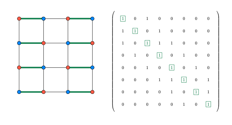
22. In How Many Ways Can
a Man Tile a Board?
\(\operatorname{per}(B_G) := \sum_{\pi \in S_n} b_{1, \pi(1)} b_{2, \pi(2)} \cdots b_{n, \pi(n)}\)
\(\operatorname{det}(B_G) := \sum_{\pi \in S_n} b_{1, \pi(1)} b_{2, \pi(2)} \cdots b_{n, \pi(n)} \cdot {\color{IndianRed}(-1)^{\operatorname{sgn}(\pi)}} \)

22. In How Many Ways Can
a Man Tile a Board?
\(\operatorname{per}(B_G) := \sum_{\pi \in S_n} b_{1, \pi(1)} b_{2, \pi(2)} \cdots b_{n, \pi(n)}\)
\(\operatorname{det}(B_G) := \sum_{\pi \in S_n} b_{1, \pi(1)} b_{2, \pi(2)} \cdots b_{n, \pi(n)} \cdot {\color{IndianRed}(-1)^{\operatorname{sgn}(\pi)}} \)

22. In How Many Ways Can
a Man Tile a Board?
\(\operatorname{per}(B_G) := \sum_{\pi \in S_n} b_{1, \pi(1)} b_{2, \pi(2)} \cdots b_{n, \pi(n)}\)
\(\operatorname{det}(B_G) := \sum_{\pi \in S_n} b_{1, \pi(1)} b_{2, \pi(2)} \cdots b_{n, \pi(n)} \cdot {\color{IndianRed}(-1)^{\operatorname{sgn}(\pi)}} \)

22. In How Many Ways Can
a Man Tile a Board?
\(\operatorname{per}(B_G) := \sum_{\pi \in S_n} b_{1, \pi(1)} b_{2, \pi(2)} \cdots b_{n, \pi(n)}\)
\(\operatorname{det}(B_G) := \sum_{\pi \in S_n} b_{1, \pi(1)} b_{2, \pi(2)} \cdots b_{n, \pi(n)} \cdot {\color{IndianRed}(-1)^{\operatorname{sgn}(\pi)}} \)
Let \(C\) be a cycle in a bipartite graph \(G\).
Then \(C\) has an even length, which we write as \(2 \ell\).
Let \(\sigma\) be a signing of \(G\), and
let \(n_C\) be the number of negative edges (i.e., edges with sign -1 ) in \(C\).
Then we call \(C\) properly signed with respect to \(\sigma\) if \(n_C \equiv \ell-1(\bmod 2)\).
A properly signed cycle of length \(4,8,12, \ldots \) contains an odd number of negative edges,
while a properly signed cycles of length \(6,10,14, \ldots\) contains an even number of negative edges.
22. In How Many Ways Can
a Man Tile a Board?
\(\operatorname{per}(B_G) := \sum_{\pi \in S_n} b_{1, \pi(1)} b_{2, \pi(2)} \cdots b_{n, \pi(n)}\)
\(\operatorname{det}(B_G) := \sum_{\pi \in S_n} b_{1, \pi(1)} b_{2, \pi(2)} \cdots b_{n, \pi(n)} \cdot {\color{IndianRed}(-1)^{\operatorname{sgn}(\pi)}} \)
Lemma A. Suppose that \(\sigma\) is a signing of a bipartite graph \(G\) (no planarity assumed here) such that every evenly placed cycle in \(G\) is properly signed.
Then \(\sigma\) is a Kasteleyn signing for \(G\).
A cycle \(C\) is evenly placed if the graph obtained from \(G\)
by deleting all vertices of \(C\) (and the adjacent edges) has a perfect matching.
22. In How Many Ways Can
a Man Tile a Board?
\(\operatorname{per}(B_G) := \sum_{\pi \in S_n} b_{1, \pi(1)} b_{2, \pi(2)} \cdots b_{n, \pi(n)}\)
\(\operatorname{det}(B_G) := \sum_{\pi \in S_n} b_{1, \pi(1)} b_{2, \pi(2)} \cdots b_{n, \pi(n)} \cdot {\color{IndianRed}(-1)^{\operatorname{sgn}(\pi)}} \)
Lemma B. Let \(G\) be a planar bipartite graph that is both connected and 2-connected, and let us fix a planar drawing of \(G\).
If \(\sigma\) is a signing of \(G\) such that the boundary cycle of every inner face in the drawing is properly signed, then \(\sigma\) is a Kasteleyn signing.
2-connected graphs: every edge belongs to a cycle.
22. In How Many Ways Can
a Man Tile a Board?
\(\operatorname{per}(B_G) := \sum_{\pi \in S_n} b_{1, \pi(1)} b_{2, \pi(2)} \cdots b_{n, \pi(n)}\)
\(\operatorname{det}(B_G) := \sum_{\pi \in S_n} b_{1, \pi(1)} b_{2, \pi(2)} \cdots b_{n, \pi(n)} \cdot {\color{IndianRed}(-1)^{\operatorname{sgn}(\pi)}} \)

22. In How Many Ways Can
a Man Tile a Board?

22. In How Many Ways Can
a Man Tile a Board?
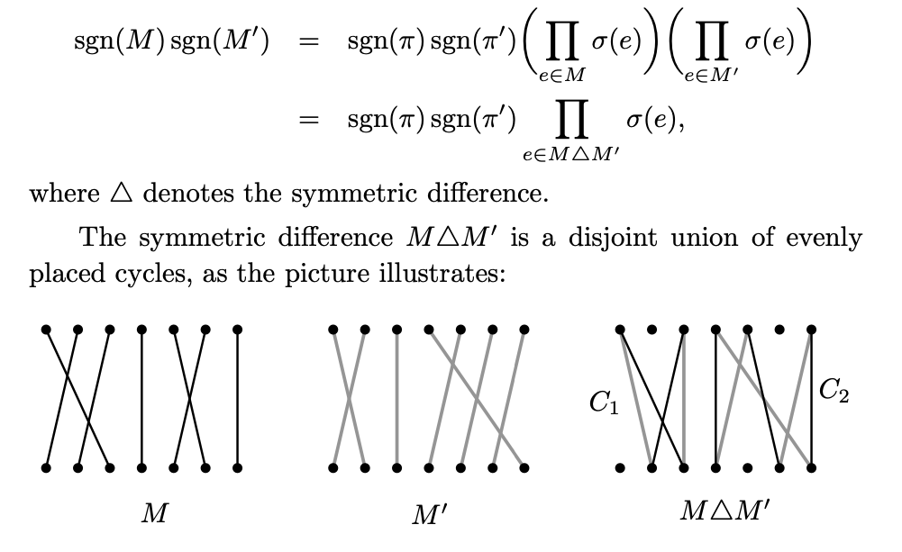
22. In How Many Ways Can
a Man Tile a Board?

12345678910111213141516\(\begin{pmatrix} 1 & 0 & 1 & 0 & 0 & 0 & 0 & 0 \\ 1 & 1 & 0 & 1 & 0 & 0 & 0 & 0 \\ 1 & 0 & 1 & 1 & 1 & 0 & 0 & 0 \\ 0 & 1 & 0 & 1 & 0 & 1 & 0 & 0 \\ 0 & 0 & 1 & 0 & 1 & 0 & 1 & 0 \\ 0 & 0 & 0 & 1 & 1 & 1 & 0 & 1 \\ 0 & 0 & 0 & 0 & 1 & 0 & 1 & 1 \\ 0 & 0 & 0 & 0 & 0 & 1 & 0 & 1 \\ \end{pmatrix}\)
1
3
6
8
9
11
14
16
2
4
5
7
10
12
13
15
22. In How Many Ways Can
a Man Tile a Board?
12345678910111213141516\(\begin{pmatrix} {\color{SeaGreen}1} & 0 & 1 & 0 & 0 & 0 & 0 & 0 \\ 1 & {\color{SeaGreen}1} & 0 & 1 & 0 & 0 & 0 & 0 \\ 1 & 0 & {\color{SeaGreen}1} & 1 & 1 & 0 & 0 & 0 \\ 0 & 1 & 0 & {\color{SeaGreen}1} & 0 & 1 & 0 & 0 \\ 0 & 0 & 1 & 0 & {\color{SeaGreen}1} & 0 & 1 & 0 \\ 0 & 0 & 0 & 1 & 1 & {\color{SeaGreen}1} & 0 & 1 \\ 0 & 0 & 0 & 0 & 1 & 0 & {\color{SeaGreen}1} & 1 \\ 0 & 0 & 0 & 0 & 0 & 1 & 0 & {\color{SeaGreen}1} \\ \end{pmatrix}\)
1
3
6
8
9
11
14
16
2
4
5
7
10
12
13
15
22. In How Many Ways Can
a Man Tile a Board?
12345678910111213141516\(\begin{pmatrix} {\color{SeaGreen}1} & 0 & 1 & 0 & 0 & 0 & 0 & 0 \\ 1 & {\color{SeaGreen}1} & 0 & 1 & 0 & 0 & 0 & 0 \\ 1 & 0 & {\color{SeaGreen}1} & 1 & 1 & 0 & 0 & 0 \\ 0 & 1 & 0 & 1 & 0 & {\color{SeaGreen}1} & 0 & 0 \\ 0 & 0 & 1 & 0 & {\color{SeaGreen}1} & 0 & 1 & 0 \\ 0 & 0 & 0 & {\color{SeaGreen}1} & 1 & 1 & 0 & 1 \\ 0 & 0 & 0 & 0 & 1 & 0 & {\color{SeaGreen}1} & 1 \\ 0 & 0 & 0 & 0 & 0 & 1 & 0 & {\color{SeaGreen}1} \\ \end{pmatrix}\)
1
3
6
8
9
11
14
16
2
4
5
7
10
12
13
15
23. More Bricks,
More Walls?

\(p_{w,h}(k)\): the #of non-increasing walls we can build
with \(k\) bricks within a box of height \(h\) and width \(w\).
23. More Bricks,
More Walls?
Theorem. For every \(w \geq 1\) and \(h \geq 1\) we have
\(p_{w, h}(0) \leq p_{w, h}(1) \leq \cdots \leq p_{w, h}\left(\left\lfloor\frac{w h}{2}\right\rfloor\right)\)
and
\(p_{w, h}\left(\left\lceil\frac{w h}{2}\right\rceil\right) \geq p_{w, h}\left(\left\lceil\frac{w h}{2}\right\rceil+1\right) \geq \cdots \geq p_{w, h}(w h-1) \geq p_{w, h}(w h).\)
That is, \(p_{w, h}(k)\) as a function of \(k\)
is nondecreasing for \(k \leq \frac{w h}{2}\) and nonincreasing for \(k \geq \frac{w h}{2}\).
23. More Bricks,
More Walls?
\(p_{w, h}(0) \leq p_{w, h}(1) \leq \cdots \leq p_{w, h}\left(\left\lfloor\frac{w h}{2}\right\rfloor\right)\)
\(\Downarrow\)
\(p_{w, h}\left(\left\lceil\frac{w h}{2}\right\rceil\right) \geq p_{w, h}\left(\left\lceil\frac{w h}{2}\right\rceil+1\right) \geq \cdots \geq p_{w, h}(w h-1) \geq p_{w, h}(w h).\)
\( p_{w, h}(k) = p_{w, h}(wh-k)\)

23. More Bricks,
More Walls?
To prove the theorem, we will show that
\({\color{IndianRed}p_{w, h}(k) \leq p_{w, h}(\ell)}\) for \(0 \leq k<\ell \leq \frac{n}{2}\).
The first step is to view a wall in the box as an equivalence class. Namely, we start with an arbitrary set of k bricks filling some k squares in the box, and then we tidy them up into a nonincreasing wall:
Let us write \(n := wh\) for the area of the box, and
let us fix a numbering of the \(n\) squares in the box by the numbers
\(1,2,...,n\).
23. More Bricks,
More Walls?

23. More Bricks,
More Walls?
23. More Bricks,
More Walls?
Non-column breaking permutation

Two subsets \(K, K^{\prime} \in \mathcal{K}\) are wall-equivalent exactly if
\(K^{\prime}=\pi(K)\)
for some permutation that doesn't break columns.
23. More Bricks,
More Walls?
Let the equivalence classes be \(\mathcal{K}_1, \mathcal{K}_2, \ldots, \mathcal{K}_r\), where \(r:=p_{w, h}(k)\).
Let \(\mathcal{L}\) be the set of all \(\ell\)-element subsets of \(\{1,2, \ldots, n\}\), and let it be divided similarly into \(s:=p_{w, h}(\ell)\) classes \(\mathcal{L}_1, \ldots, \mathcal{L}_s\) according to wall-equivalence.
Recall: \(0 \leq k<\ell \leq \frac{n}{2}\)
The goal is to prove that \(r \leq s\).
23. More Bricks,
More Walls?
Let us consider the bipartite graph \(G\) with vertex set \(\mathcal{K} \cup \mathcal{L}\) and with edges corresponding to inclusion;
i.e., a \(k\)-element set \(K \in \mathcal{K}\) is connected to an \(\ell\)-element set \(L \in \mathcal{L}\)
by an edge if \(K \subseteq L\).

\(K_i \in \mathcal{K}\)
23. More Bricks,
More Walls?
Consider a partitioned bipartite graph that is \(V\)-degree-homogeneous.
\(U\)
\(V\)
\(V_j\)
\(U_i\)
All \(v \in V_j\) have \(d_{ij}\) neighbors in \(U_i\).
\(\longleftarrow r \longrightarrow\)
\(\longleftarrow s \longrightarrow\)
23. More Bricks,
More Walls?
Lemma. Let \(G\) be a \(V\)-homogeneous bipartite graph as below and suppose that
the rows of the matrix \(B\) are linearly independent. Then \(r \leq s\).
\(U\)
\(V\)
\(V_j\)
\(U_i\)
\(b_{u v}:= \begin{cases}1 & \text { if }\{u, v\} \in E(G) \\ 0 & \text { otherwise. }\end{cases}\)
\(\longleftarrow r \longrightarrow\)
\(\longleftarrow s \longrightarrow\)
23. More Bricks,
More Walls?
(Gottlieb's theorem.) For \(0 \leq k<\ell \leq \frac{n}{2}\), the zero-one matrix \(B\) with:
rows indexed by \(\mathcal{K}\) (all \(k\)-subsets of \(\{1,2, \ldots, n\}\) ),
columns indexed by \(\mathcal{L}\) (all \(\ell\)-subsets of \(\{1,2, \ldots, n\}\)),
and the nonzero entries corresponding to containment,
has linearly independent rows.
23. More Bricks,
More Walls?

23. More Bricks,
More Walls?
Suppose, for the sake of contradiction, that
there is a non-zero \(\mathbf{y}\) such that \(\mathbf{y}^TB = 0\).
Fix some \(K_0 \in \mathcal{K}\) with \(y_{K_0} \neq 0\).
\(\begin{array}{ll}\mathcal{K}_i:=\left\{K \in \mathcal{K}:\left|K \cap K_0\right|=i\right\}, & i=0,1, \ldots, k \\ ~\\ \mathcal{L}_j:=\left\{L \in \mathcal{L}:\left|L \cap K_0\right|=j\right\}, & j=0,1, \ldots, k\end{array}\)
Every \(K \in \mathcal{K}_i\) has the same number \(d_{i j}\) of neighbors in \(\mathcal{L}_j\).
More explicitly, \(d_{i j}\) is the number of ways of extending a \(k\)-element set \(K\) with \(\left|K \cap K_0\right|=i\) to an \(\ell\)-element \(L \supset K\) with \(\left|L \cap K_0\right|=j\).
23. More Bricks,
More Walls?
Every \(K \in \mathcal{K}_i\) has the same number \(d_{i j}\) of neighbors in \(\mathcal{L}_j\).
More explicitly, \(d_{i j}\) is the number of ways of extending a \(k\)-element set \(K\) with \(\left|K \cap K_0\right|=i\) to an \(\ell\)-element \(L \supset K\) with \(\left|L \cap K_0\right|=j\).
By this description, we have \(d_{i j}=0\) for \(i>j\).
The \(\mathcal{K}\)-degree matrix \(D\) is upper triangular.
Moreover, \(d_{i i} \neq 0\) for all \(i=0,1, \ldots, k\).
So \(D\) is non-singular.
Goal. Show the existence of a non-zero \(\mathbf{x}\) for which: \(\mathbf{x}^T D=\mathbf{0}\)
\(x_i:=\sum_{K \in \mathcal{K}_i} y_K\)
23. More Bricks,
More Walls?
By this description, we have \(d_{i j}=0\) for \(i>j\).
The \(\mathcal{K}\)-degree matrix \(D\) is upper triangular.
Moreover, \(d_{i i} \neq 0\) for all \(i=0,1, \ldots, k\).
So \(D\) is non-singular.
Goal. Show the existence of a non-zero \(\mathbf{x}\) for which: \(\mathbf{x}^T D=\mathbf{0}\)
\(x_i:=\sum_{K \in \mathcal{K}_i} y_K\)
\(\begin{aligned} 0 & =\sum_{L \in \mathcal{L}_j}\left(\mathbf{y}^T B\right)_L=\sum_{L \in \mathcal{L}_j} \sum_{K \in \mathcal{K}} y_K b_{K L}=\sum_{K \in \mathcal{K}} y_K \sum_{L \in \mathcal{L}_j} b_{K L} \\ & =\sum_{i=0}^k \sum_{K \in \mathcal{K}_i} y_K d_{i j}=\sum_{i=0}^k x_i d_{i j}=\left(\mathbf{x}^T D\right)_j .\end{aligned}\)
24. Perfect Matchings and Determinants
A matching in a graph \(G\) is a set of edges \(F \subseteq E(G)\) such that no vertex of \(G\) is incident to more than one edge of \(F\).
A perfect matching is a matching covering all vertices.

Goal. A randomized algorithm for detecting perfect matchings.
24. Perfect Matchings and Determinants
Consider a bipartite graph \(G\).
Its vertices are divided into two classes \(\left\{u_1, u_2, \ldots, u_n\right\}\) and \(\left\{v_1, v_2, \ldots, v_n\right\}\)
...and the edges go only between the two classes.
\(\begin{pmatrix}\small{1} & \small{0} & \small{1} & \small{0} & \small{0} \\ \small{0} & \small{1} & \small{0} & \small{1} & \small{0} \\ \small{1} & \small{0} & \small{0} & \small{0} & \small{1} \\ \small{0} & \small{1} & \small{0} & \small{0} & \small{0} \\ \small{0} & \small{0} & \small{1} & \small{0} & \small{1} \\ \end{pmatrix}\)
24. Perfect Matchings and Determinants
Let \(S_n\) be the set of all permutations of the set \(\{1,2, \ldots, n\}\).
We can describe it as
\(\left\{\left\{u_1, v_{\pi(1)}\right\},\left\{u_2, v_{\pi(2)}\right\}, \ldots\right.\), \(\left.\left\{u_n, v_{\pi(n)}\right\}\right\}\)
\(\begin{pmatrix}\small{1} & \small{0} & \small{1} & \small{0} & \small{0} \\ \small{0} & \small{1} & \small{0} & \small{1} & \small{0} \\ \small{1} & \small{0} & \small{0} & \small{0} & \small{1} \\ \small{0} & \small{1} & \small{0} & \small{0} & \small{0} \\ \small{0} & \small{0} & \small{1} & \small{0} & \small{1} \\ \end{pmatrix}\)
Every perfect matching of \(G\)
uniquely corresponds to a permutation \(\pi \in S_n\).
1
2
3
4
5
1
2
3
4
5
24. Perfect Matchings and Determinants
Let \(S_n\) be the set of all permutations of the set \(\{1,2, \ldots, n\}\).
We can describe it as
\(\left\{(1,3),(2,4),(3,1),(4,2),(5,5)\right\}\)
\(\begin{pmatrix}\small{1} & \small{0} & \small{1} & \small{0} & \small{0} \\ \small{0} & \small{1} & \small{0} & \small{1} & \small{0} \\ \small{1} & \small{0} & \small{0} & \small{0} & \small{1} \\ \small{0} & \small{1} & \small{0} & \small{0} & \small{0} \\ \small{0} & \small{0} & \small{1} & \small{0} & \small{1} \\ \end{pmatrix}\)
Every perfect matching of \(G\)
uniquely corresponds to a permutation \(\pi \in S_n\).
1
2
3
4
5
1
2
3
4
5
24. Perfect Matchings and Determinants
Let \(S_n\) be the set of all permutations of the set \(\{1,2, \ldots, n\}\).
We can describe it as
\(\left\{(1,1),(2,4),(3,5),(4,2),(5,3)\right\}\)
\(\begin{pmatrix}\small{1} & \small{0} & \small{1} & \small{0} & \small{0} \\ \small{0} & \small{1} & \small{0} & \small{1} & \small{0} \\ \small{1} & \small{0} & \small{0} & \small{0} & \small{1} \\ \small{0} & \small{1} & \small{0} & \small{0} & \small{0} \\ \small{0} & \small{0} & \small{1} & \small{0} & \small{1} \\ \end{pmatrix}\)
Every perfect matching of \(G\)
uniquely corresponds to a permutation \(\pi \in S_n\).
1
2
3
4
5
1
2
3
4
5
24. Perfect Matchings and Determinants
\(a_{i j}:= \begin{cases}x_{i j} & \text { if }\left\{u_i, v_j\right\} \in E(G) \\ 0 & \text { otherwise }\end{cases}\)
\(\begin{pmatrix} \small{x_{11}} & \small{0} & \small{x_{13}} & \small{0} & \small{0} \\ \small{0} & \small{x_{22}} & \small{0} & \small{x_{24}} & \small{0} \\ \small{x_{31}} & \small{0} & \small{0} & \small{0} & \small{x_{35}} \\ \small{0} & \small{x_{42}} & \small{0} & \small{0} & \small{0} \\ \small{0} & \small{0} & \small{x_{53}} & \small{0} & \small{x_{55}} \\ \end{pmatrix}\)

\(\operatorname{det}(A) = x_{24}x_{42}x_{11}x_{53}x_{35} + x_{24}x_{42}x_{31}x_{55}x_{13}\)
24. Perfect Matchings and Determinants
\(a_{i j}:= \begin{cases}x_{i j} & \text { if }\left\{u_i, v_j\right\} \in E(G) \\ 0 & \text { otherwise }\end{cases}\)
\(\begin{aligned}\operatorname{det}(A) & =\sum_{\pi \in S_n} \operatorname{sgn}(\pi) \cdot a_{1, \pi(1)} a_{2, \pi(2)} \cdots a_{n, \pi(n)} \\& =\sum_{\substack{\pi \text { describes a perfect } \\\text { matching of } G}} \operatorname{sgn}(\pi) \cdot x_{1, \pi(1)} x_{2, \pi(2)} \cdots x_{n, \pi(n)} .\end{aligned}\)
\(\begin{pmatrix} \small{x_{11}} & \small{0} & \small{x_{13}} & \small{0} & \small{0} \\ \small{0} & \small{x_{22}} & \small{0} & \small{x_{24}} & \small{0} \\ \small{x_{31}} & \small{0} & \small{0} & \small{0} & \small{x_{35}} \\ \small{0} & \small{x_{42}} & \small{0} & \small{0} & \small{0} \\ \small{0} & \small{0} & \small{x_{53}} & \small{0} & \small{x_{55}} \\ \end{pmatrix}\)
24. Perfect Matchings and Determinants
\(a_{i j}:= \begin{cases}x_{i j} & \text { if }\left\{u_i, v_j\right\} \in E(G) \\ 0 & \text { otherwise }\end{cases}\)
\(\begin{aligned}\operatorname{det}(A) & =\sum_{\pi \in S_n} \operatorname{sgn}(\pi) \cdot a_{1, \pi(1)} a_{2, \pi(2)} \cdots a_{n, \pi(n)} \\& =\sum_{\substack{\pi \text { describes a perfect } \\\text { matching of } G}} \operatorname{sgn}(\pi) \cdot x_{1, \pi(1)} x_{2, \pi(2)} \cdots x_{n, \pi(n)} .\end{aligned}\)
Lemma. The polynomial \(\operatorname{det}(A)\) is identically zero
if and only if
\(G\) has no a perfect matching.
24. Perfect Matchings and Determinants
\(a_{i j}:= \begin{cases}x_{i j} & \text { if }\left\{u_i, v_j\right\} \in E(G) \\ 0 & \text { otherwise }\end{cases}\)
\(\begin{aligned}\operatorname{det}(A) & =\sum_{\pi \in S_n} \operatorname{sgn}(\pi) \cdot a_{1, \pi(1)} a_{2, \pi(2)} \cdots a_{n, \pi(n)} \\& =\sum_{\substack{\pi \text { describes a perfect } \\\text { matching of } G}} \operatorname{sgn}(\pi) \cdot x_{1, \pi(1)} x_{2, \pi(2)} \cdots x_{n, \pi(n)} .\end{aligned}\)
Lemma. The polynomial \(\operatorname{det}(A)\) is identically zero
\(\Uparrow\)
\(G\) has no a perfect matching.
24. Perfect Matchings and Determinants
\(a_{i j}:= \begin{cases}x_{i j} & \text { if }\left\{u_i, v_j\right\} \in E(G) \\ 0 & \text { otherwise }\end{cases}\)
\(\begin{aligned}\operatorname{det}(A) & =\sum_{\pi \in S_n} \operatorname{sgn}(\pi) \cdot a_{1, \pi(1)} a_{2, \pi(2)} \cdots a_{n, \pi(n)} \\& =\sum_{\substack{\pi \text { describes a perfect } \\\text { matching of } G}} \operatorname{sgn}(\pi) \cdot x_{1, \pi(1)} x_{2, \pi(2)} \cdots x_{n, \pi(n)} .\end{aligned}\)
Lemma. The polynomial \(\operatorname{det}(A)\) is identically zero
\(\Downarrow\)
\(G\) has no a perfect matching.
24. Perfect Matchings and Determinants
\(a_{i j}:= \begin{cases}x_{i j} & \text { if }\left\{u_i, v_j\right\} \in E(G) \\ 0 & \text { otherwise }\end{cases}\)
\(\begin{aligned}\operatorname{det}(A) & =\sum_{\pi \in S_n} \operatorname{sgn}(\pi) \cdot a_{1, \pi(1)} a_{2, \pi(2)} \cdots a_{n, \pi(n)}\end{aligned}\)
\(\operatorname{det}(A)\) is identically zero \(\equiv\) \(G\) has no a perfect matching.
Now we would like to test whether the polynomial \(\operatorname{det}(A)\) is the zero polynomial.
We can't afford to compute it explicitly as a polynomial, since it has the same number of terms as the number of perfect matchings of \(G\) and that can be exponentially many.
24. Perfect Matchings and Determinants
\(a_{i j}:= \begin{cases}x_{i j} & \text { if }\left\{u_i, v_j\right\} \in E(G) \\ 0 & \text { otherwise }\end{cases}\)
\(\begin{aligned}\operatorname{det}(A) & =\sum_{\pi \in S_n} \operatorname{sgn}(\pi) \cdot a_{1, \pi(1)} a_{2, \pi(2)} \cdots a_{n, \pi(n)}\end{aligned}\)
\(\operatorname{det}(A)\) is identically zero \(\equiv\) \(G\) has no a perfect matching.
Now we would like to test whether the polynomial \(\operatorname{det}(A)\) is the zero polynomial.
But if we substitute any specific numbers for the variables \(x_{i j}\), we can easily calculate the determinant, e.g., by the Gaussian elimination.
So we can imagine that \(\operatorname{det}(A)\) is available to us through a black box,
from which we can obtain the value of the polynomial at any specified point.
24. Perfect Matchings and Determinants
\(a_{i j}:= \begin{cases}x_{i j} & \text { if }\left\{u_i, v_j\right\} \in E(G) \\ 0 & \text { otherwise }\end{cases}\)
\(\begin{aligned}\operatorname{det}(A) & =\sum_{\pi \in S_n} \operatorname{sgn}(\pi) \cdot a_{1, \pi(1)} a_{2, \pi(2)} \cdots a_{n, \pi(n)}\end{aligned}\)
\(\operatorname{det}(A)\) is identically zero \(\equiv\) \(G\) has no a perfect matching.
For an arbitrary function given by a black box, we can never be sure that it is identically 0 unless we check its values at all points.
But a polynomial has a wonderful property:
Either it equals \(0\) everywhere, or almost nowhere.
24. Perfect Matchings and Determinants
Theorem (Roots of a degree d polynomial).
Let \(\mathbb{K}\) be an arbitrary field, and let \(S\) be a finite subset of \(\mathbb{K}\).
Then for every non-zero polynomial
\(p\left(x\right)\) of degree \(d\) in one variable and with coefficients from \(\mathbb{K}\),
the number of \(r \in S\) with \(p\left(r\right)=0\)
is at most \(d\).
In other words, if \(r \in S\) are chosen independently and uniformly at random, then the probability of \(p\left(r\right)=0\) is at most \(\frac{d}{|S|}\).
24. Perfect Matchings and Determinants
Theorem (The Schwartz-Zippel theorem).
Let \(\mathbb{K}\) be an arbitrary field, and let \(S\) be a finite subset of \(\mathbb{K}\).
Then for every non-zero polynomial
\(p\left(x_1, \ldots, x_m\right)\) of degree \(d\) in \(m\) variables and with coefficients from \(\mathbb{K}\),
the number of \(m\)-tuples \(\left(r_1, r_2, \ldots, r_m\right) \in S^m\) with \(p\left(r_1, r_2, \ldots, r_m\right)=0\)
is at most \(d|S|^{m-1}\).
In other words, if \(r_1, r_2, \ldots\), \(r_m \in S\) are chosen independently and uniformly at random, then the probability of \(p\left(r_1, r_2, \ldots, r_m\right)=0\) is at most \(\frac{d}{|S|}\).
24. Perfect Matchings and Determinants
\(\neq 0\)
Pick \(r_1, r_2, \ldots\), \(r_m \in S\) u.a.r.
\(= 0\)
\(\operatorname{det}(A_{[x_{\ell} = r_\ell]})\)
Correctly
conclude that
\(G\) has a
perfect matching.
Conclude that
\(G\) does not
have any
perfect matching
w.h.p.
(Graphs without PMs are detected accurately;
graphs with PMs may be problematic.)
If \(r_1, r_2, \ldots\), \(r_m \in S\) are chosen independently and uniformly at random, then the probability of \(p\left(r_1, r_2, \ldots, r_m\right)=0\) is at most \(\frac{d}{|S|} = {\color{SeaGreen}\frac{1}{2}}\).
24. Perfect Matchings and Determinants
Theorem (The Schwartz-Zippel theorem).
Let \(\mathbb{K}\) be an arbitrary field, and let \(S\) be a finite subset of \(\mathbb{K}\).
Then for every non-zero polynomial
\(p\left(x_1, \ldots, x_m\right)\) of degree \(d\) in \(m\) variables and with coefficients from \(\mathbb{K}\),
the number of \(m\)-tuples \(\left(r_1, r_2, \ldots, r_m\right) \in S^m\) with \(p\left(r_1, r_2, \ldots, r_m\right)=0\)
is at most \(d|S|^{m-1}\).
In other words, if \(r_1, r_2, \ldots\), \(r_m \in S\) are chosen independently and uniformly at random, then the probability of \(p\left(r_1, r_2, \ldots, r_m\right)=0\) is at most \(\frac{d}{|S|}\).
24. Perfect Matchings and Determinants
Let \(m>1\). Let us suppose that \(x_1\) occurs in at least one term of \(p\left(x_1, \ldots, x_n\right)\) with a nonzero coefficient.
Let us write \(p\left(x_1, \ldots, x_m\right)\) as a polynomial in \(x_1\)
with coefficients being polynomials in \(x_2, \ldots, x_n\) :
\(p\left(x_1, x_2, \ldots, x_m\right)=\sum_{i=0}^k x_1^i p_i\left(x_2, \ldots, x_m\right),\)
where \(k\) is the maximum exponent of \(x_1\) in \(p\left(x_1, \ldots, x_n\right)\).
\({\color{IndianRed}x_1^0}(x_3^2x_5x_7) + {\color{IndianRed}x_1^1}(x_2x_3^2 + x_5x_6x_7) + {\color{IndianRed}x_1^2}(x_3x_5 + x_4x_2^4) + \cdots + {\color{IndianRed}x_1^7}(x_2x_6 + x_3^3x_5^5)\)
\(R_1 := \{(r_1,\ldots,r_m)~\vert~{\color{IndianRed}p\left(r_1, r_2, \ldots, r_m\right)=0}, {\color{SeaGreen}p_k\left(r_2, \ldots, r_m\right)=0}\}\)
Since the polynomial \(p_k\left(x_2, \ldots, x_m\right)\) is not identically zero and has degree at most \(d-k\),
the number of choices for \(\left(r_2, \ldots, r_m\right)\) is at most \((d-k)|S|^{m-2}\) by the induction hypothesis,
and so \(\left|R_1\right| \leq\) \((d-k)|S|^{m-1}\)
24. Perfect Matchings and Determinants
Let \(m>1\). Let us suppose that \(x_1\) occurs in at least one term of \(p\left(x_1, \ldots, x_n\right)\) with a nonzero coefficient.
Let us write \(p\left(x_1, \ldots, x_m\right)\) as a polynomial in \(x_1\)
with coefficients being polynomials in \(x_2, \ldots, x_n\) :
\(p\left(x_1, x_2, \ldots, x_m\right)=\sum_{i=0}^k x_1^i p_i\left(x_2, \ldots, x_m\right),\)
where \(k\) is the maximum exponent of \(x_1\) in \(p\left(x_1, \ldots, x_n\right)\).
\({\color{IndianRed}x_1^0}(x_3^2x_5x_7) + {\color{IndianRed}x_1^1}(x_2x_3^2 + x_5x_6x_7) + {\color{IndianRed}x_1^2}(x_3x_5 + x_4x_2^4) + \cdots + {\color{IndianRed}x_1^7}(x_2x_6 + x_3^3x_5^5)\)
\(R_2 := \{(r_1,\ldots,r_m)~\vert~{\color{IndianRed}p\left(r_1, r_2, \ldots, r_m\right)=0}, {\color{SeaGreen}p_k\left(r_2, \ldots, r_m\right)\neq0}\}\)
Here, \(r_2\) through \(r_m\) can be chosen in at most \(|S|^{m-1}\) ways, and if \(r_2, \ldots, r_m\) are fixed with \(p_k\left(r_2, \ldots, r_m\right) \neq 0\), then \(r_1\) must be a root of the univariate polynomial \(q\left(x_1\right)=p\left(x_1, {\color{Tomato}r_2, \ldots, r_m}\right)\). This polynomial has degree (exactly) \(k\), and hence it has at most \(k\) roots.
Thus the second class has at most \(k|S|^{m-1} m\)-tuples.
25. Turning a ladder over a finite field

A Kakeya set, or Besicovitch set, is a set of points in Euclidean space which contains a unit line segment in every direction.
A Kakeya needle set (sometimes also known as a Kakeya set)
is a (Besicovitch) set in the plane with a stronger property, that a unit line segment can be rotated continuously through 180 degrees within it, returning to its original position with reversed orientation.
25. Turning a ladder over a finite field
A set \(K\) in the vector space \(\mathbb{F}^n\) is a Kakeya set if it contains a line in every possible direction;
that is, for every nonzero \({\color{IndianRed}\mathbf{u} \in \mathbb{F}^n}\) there is
\(\mathbf{a} \in \mathbb{F}^n\) such that \({\color{SeaGreen}\mathbf{a}+t \mathbf{u}}\) belongs to \(K\) for all \(t \in \mathbb{F}\).
25. Turning a ladder over a finite field

25. Turning a ladder over a finite field

25. Turning a ladder over a finite field

25. Turning a ladder over a finite field

25. Turning a ladder over a finite field

25. Turning a ladder over a finite field

25. Turning a ladder over a finite field
A set \(K\) in the vector space \(\mathbb{F}^n\) is a Kakeya set if it contains a line in every possible direction;
that is, for every nonzero \({\color{IndianRed}\mathbf{u} \in \mathbb{F}^n}\) there is
\(\mathbf{a} \in \mathbb{F}^n\) such that \({\color{SeaGreen}\mathbf{a}+t \mathbf{u}}\) belongs to \(K\) for all \(t \in \mathbb{F}\).
Proposition. Any Kakeya set in \(\mathbb{F}_q^2\) contains at least \(\frac{1}{2} q^2\) points.
How small can a Kakeya set be?
Proof. The first line has \(q\) points, the second adds at least \(q-1\) new points, the third adds at least \(q-2\) more, ..., yielding at least \(\frac{q(q+1)}{2}>\frac{1}{2} q^2\) points in total.
25. Turning a ladder over a finite field
A set \(K\) in the vector space \(\mathbb{F}^n\) is a Kakeya set if it contains a line in every possible direction;
that is, for every nonzero \({\color{IndianRed}\mathbf{u} \in \mathbb{F}^n}\) there is
\(\mathbf{a} \in \mathbb{F}^n\) such that \({\color{SeaGreen}\mathbf{a}+t \mathbf{u}}\) belongs to \(K\) for all \(t \in \mathbb{F}\).
Theorem (Kakeya's conjecture for finite fields). Let \(\mathbb{F}\) be a \(q\)-element field. Then any Kakeya set \(K\) in \(\mathbb{F}^n\) has at least \(\left(\begin{array}{c}q+n-1 \\ n\end{array}\right)\) elements.
How small can a Kakeya set be?
25. Turning a ladder over a finite field
A set \(K\) in the vector space \(\mathbb{F}^n\) is a Kakeya set if for every nonzero \({\color{IndianRed}\mathbf{u} \in \mathbb{F}^n}\) there is
\(\mathbf{a} \in \mathbb{F}^n\) such that \({\color{SeaGreen}\mathbf{a}+t \mathbf{u}}\) belongs to \(K\) for all \(t \in \mathbb{F}\).
Theorem Let \(\mathbb{F}\) be a q-element field.
Then any Kakeya set \(K\) in \(\mathbb{F}^n\) has at least \(\left(\begin{array}{c}q+n-1 \\ n\end{array}\right)\) elements.
Lemma. Let \(\mathbf{a}_1, \mathbf{a}_2, \ldots, \mathbf{a}_N\) be points in \(\mathbb{F}^n\), where \(N<\left(\begin{array}{c}d+n \\ n\end{array}\right)\). Then there exists a nonzero polynomial \(p\left(x_1, x_2, \ldots, x_n\right)\) of degree at most \(d\) such that \(p\left(\mathbf{a}_i\right)=0\) for all \(i\).
25. Turning a ladder over a finite field
A set \(K\) in the vector space \(\mathbb{F}^n\) is a Kakeya set if for every nonzero \({\color{IndianRed}\mathbf{u} \in \mathbb{F}^n}\) there is
\(\mathbf{a} \in \mathbb{F}^n\) such that \({\color{SeaGreen}\mathbf{a}+t \mathbf{u}}\) belongs to \(K\) for all \(t \in \mathbb{F}\).
We proceed by contradiction, assuming \(|K|<\left(\begin{array}{c}n+q-1 \\ n\end{array}\right)\).
Then there is a nonzero polynomial \(p\) of degree \(d \leq q-1\) vanishing at all points of \(K\).
Theorem Let \(\mathbb{F}\) be a q-element field.
Then any Kakeya set \(K\) in \(\mathbb{F}^n\) has at least \(\left(\begin{array}{c}q+n-1 \\ n\end{array}\right)\) elements.
25. Turning a ladder over a finite field
A set \(K\) in the vector space \(\mathbb{F}^n\) is a Kakeya set if for every nonzero \({\color{IndianRed}\mathbf{u} \in \mathbb{F}^n}\) there is
\(\mathbf{a} \in \mathbb{F}^n\) such that \({\color{SeaGreen}\mathbf{a}+t \mathbf{u}}\) belongs to \(K\) for all \(t \in \mathbb{F}\).
Theorem Let \(\mathbb{F}\) be a q-element field.
Then any Kakeya set \(K\) in \(\mathbb{F}^n\) has at least \(\left(\begin{array}{c}q+n-1 \\ n\end{array}\right)\) elements.
Then there is a nonzero polynomial \(p\) of degree \(d \leq q-1\) vanishing at all points of \(K\).
Let \(p=p_0+p_1+\cdots+p_{d}\) where \(p_i\) is homogeneous of degree \(i\).
Fix any direction \(\mathbf{u}\). Because \(p\) vanishes on a line in the direction \(\mathbf{u}\),
there exists \(\mathbf{a}\) such that \(p(\mathbf{a}+t\mathbf{u})=0\) for all \(t\) in \(\mathbb{F}_q\).
25. Turning a ladder over a finite field
A set \(K\) in the vector space \(\mathbb{F}^n\) is a Kakeya set if for every nonzero \({\color{IndianRed}\mathbf{u} \in \mathbb{F}^n}\) there is
\(\mathbf{a} \in \mathbb{F}^n\) such that \({\color{SeaGreen}\mathbf{a}+t \mathbf{u}}\) belongs to \(K\) for all \(t \in \mathbb{F}\).
Theorem Let \(\mathbb{F}\) be a q-element field.
Then any Kakeya set \(K\) in \(\mathbb{F}^n\) has at least \(\left(\begin{array}{c}q+n-1 \\ n\end{array}\right)\) elements.
Suppose we have a polynomial \(p(x_1,x_2) := x_1x_2 + x_1^2 + x_2^2 + x_1^2x_2^5\).
Suppose we have a line: \(L_{\mathbf{a},\mathbf{u}} := \{\mathbf{a}+t\mathbf{u} ~|~ t \in \mathbb{F}_5, \mathbf{a} \in \mathbb{F}^2, \mathbf{u} \in \mathbb{F}^2 \setminus \{(0,0)\}\}\).
\(L_{\mathbf{a},\mathbf{u}} := \{(a_1,a_2), (a_1 + u_1, a_2 + u_2), (a_1 + 2u_1, a_2 + 2u_2), (a_1 + 3u_1, a_2 + 3u_2), (a_1 + 4u_1, a_2 + 4u_2)\}\).
\(p(\mathbf{a}+t\mathbf{u})\) = ?
25. Turning a ladder over a finite field
A set \(K\) in the vector space \(\mathbb{F}^n\) is a Kakeya set if for every nonzero \({\color{IndianRed}\mathbf{u} \in \mathbb{F}^n}\) there is
\(\mathbf{a} \in \mathbb{F}^n\) such that \({\color{SeaGreen}\mathbf{a}+t \mathbf{u}}\) belongs to \(K\) for all \(t \in \mathbb{F}\).
Theorem Let \(\mathbb{F}\) be a q-element field.
Then any Kakeya set \(K\) in \(\mathbb{F}^n\) has at least \(\left(\begin{array}{c}q+n-1 \\ n\end{array}\right)\) elements.
Suppose we have a polynomial \(p(x_1,x_2) := x_1x_2 + x_1^2 + x_2^2 + x_1^2x_2^5\).
Suppose we have a line: \(L_{\mathbf{a},\mathbf{u}} := \{\mathbf{a}+t\mathbf{u} ~|~ t \in \mathbb{F}_5, \mathbf{a} \in \mathbb{F}^2, \mathbf{u} \in \mathbb{F}^2 \setminus \{(0,0)\}\}\).
\(L_{\mathbf{a},\mathbf{u}} := \{(a_1,a_2), (a_1 + u_1, a_2 + u_2), (a_1 + 2u_1, a_2 + 2u_2), (a_1 + 3u_1, a_2 + 3u_2), (a_1 + 4u_1, a_2 + 4u_2)\}\).
\(p(\mathbf{a}+t\mathbf{u})\) = \(p(x_1 := a_1 + tu_1, x_2 := a_2 + tu_2 )\)
\((a_1 + tu_1)(a_2 + tu_2) + (a_1 + tu_1)^2 + (a_2 + tu_2)^2 + (a_1 + tu_1)^2(a_2 + tu_2)^5\)
Coefficient of \(t^7\)?
25. Turning a ladder over a finite field
A set \(K\) in the vector space \(\mathbb{F}^n\) is a Kakeya set if for every nonzero \({\color{IndianRed}\mathbf{u} \in \mathbb{F}^n}\) there is
\(\mathbf{a} \in \mathbb{F}^n\) such that \({\color{SeaGreen}\mathbf{a}+t \mathbf{u}}\) belongs to \(K\) for all \(t \in \mathbb{F}\).
Theorem Let \(\mathbb{F}\) be a q-element field.
Then any Kakeya set \(K\) in \(\mathbb{F}^n\) has at least \(\left(\begin{array}{c}q+n-1 \\ n\end{array}\right)\) elements.
Suppose we have a polynomial \(p(x_1,x_2) := x_1x_2 + x_1^2 + x_2^2 + x_1^2x_2^5\).
Suppose we have a line: \(L_{\mathbf{a},\mathbf{u}} := \{\mathbf{a}+t\mathbf{u} ~|~ t \in \mathbb{F}_5, \mathbf{a} \in \mathbb{F}^2, \mathbf{u} \in \mathbb{F}^2 \setminus \{(0,0)\}\}\).
\(L_{\mathbf{a},\mathbf{u}} := \{(a_1,a_2), (a_1 + u_1, a_2 + u_2), (a_1 + 2u_1, a_2 + 2u_2), (a_1 + 3u_1, a_2 + 3u_2), (a_1 + 4u_1, a_2 + 4u_2)\}\).
\(p(\mathbf{a}+t\mathbf{u})\) = \(p(x_1 := a_1 + tu_1, x_2 := a_2 + tu_2 )\)
\((a_1 + tu_1)(a_2 + tu_2) + (a_1 + tu_1)^2 + (a_2 + tu_2)^2 + (a_1 + tu_1)^2(a_2 + tu_2)^5\)
\((u_1^2 \cdot u_2^5) \cdot t^7\)
25. Turning a ladder over a finite field
A set \(K\) in the vector space \(\mathbb{F}^n\) is a Kakeya set if for every nonzero \({\color{IndianRed}\mathbf{u} \in \mathbb{F}^n}\) there is
\(\mathbf{a} \in \mathbb{F}^n\) such that \({\color{SeaGreen}\mathbf{a}+t \mathbf{u}}\) belongs to \(K\) for all \(t \in \mathbb{F}\).
Theorem Let \(\mathbb{F}\) be a q-element field.
Then any Kakeya set \(K\) in \(\mathbb{F}^n\) has at least \(\left(\begin{array}{c}q+n-1 \\ n\end{array}\right)\) elements.
Then there is a nonzero polynomial \(p\) of degree \(d \leq q-1\) vanishing at all points of \(K\).
Let \(p=p_0+p_1+\cdots+p_{d}\) where \(p_i\) is homogeneous of degree \(i\).
Fix any direction \(\mathbf{u}\). Because \(p\) vanishes on a line in the direction \(\mathbf{u}\),
there exists \(\mathbf{a}\) such that \(p(\mathbf{a}+t\mathbf{u})=0\) for all \(t\) in \(\mathbb{F}_q\).
Then \(p(\mathbf{a}+t\mathbf{u})\) is a polynomial of degree at most \(q-1\) in \(t\) having \(q\) roots in \(\mathbb{F}_q\),
so it is the zero polynomial.
Coefficient of \(t^{d}\) in \(p(\mathbf{a}+t\mathbf{u})\) is \(p_{d}(\mathbf{u}) \not\equiv 0\).
But \(p_{d}(\mathbf{u}) = 0\), for all \(\mathbf{u} \in \mathbb{F}^n\).
25. Turning a ladder over a finite field
A set \(K\) in the vector space \(\mathbb{F}^n\) is a Kakeya set if for every nonzero \({\color{IndianRed}\mathbf{u} \in \mathbb{F}^n}\) there is
\(\mathbf{a} \in \mathbb{F}^n\) such that \({\color{SeaGreen}\mathbf{a}+t \mathbf{u}}\) belongs to \(K\) for all \(t \in \mathbb{F}\).
Theorem Let \(\mathbb{F}\) be a q-element field.
Then any Kakeya set \(K\) in \(\mathbb{F}^n\) has at least \(\left(\begin{array}{c}q+n-1 \\ n\end{array}\right)\) elements.
(SZ.) A nonzero polynomial of degree \(d\) can vanish on
at most \(d q^{n-1} \leqslant (q-1) q^n<\left|\mathbb{F}^n\right|\) points of \(\mathbb{F}^n\).
But \(p_{d}(\mathbf{u}) = 0\), for all \(\mathbf{u} \in \mathbb{F}^n\).
25. Turning a ladder over a finite field
Lemma. Let \(\mathbf{a}_1, \mathbf{a}_2, \ldots, \mathbf{a}_N\) be points in \(\mathbb{F}^n\), where \(N<\left(\begin{array}{c}d+n \\ n\end{array}\right)\). Then there exists a nonzero polynomial \(p\left(x_1, x_2, \ldots, x_n\right)\) of degree at most \(d\) such that \(p\left(\mathbf{a}_i\right)=0\) for all \(i\).
\(p(x_1, \ldots, x_n) := \sum_{\alpha_1+\cdots+\alpha_n \leq d} c_{\alpha_1, \ldots, \alpha_n} x_1^{\alpha_1} \cdots x_n^{\alpha_n}\)
...where the sum is over all \(n\)-tuples of nonnegative integers \(\left(\alpha_1, \ldots, \alpha_n\right)\) summing to at most \(d\), and the \(c_{\alpha_1, \ldots, \alpha_n} \in \mathbb{F}\) are coefficients.
#coefficients \(= \left(\begin{array}{c}d+n \\n\end{array}\right)\)
A requirement of the form \(p(\mathbf{a})=0\) translates to
a homogeneous linear equation with the \(c_{\alpha_1, \ldots, \alpha_n}\) as unknowns.
We have \(N\) such equations: fewer equations than unknowns.
26. Counting Compositions
A permutation is denoted as a sequence, e.g: \((2,1,5,3,4)\)
26. Counting Compositions
Permutations compose as you would expect:
\((2,1,5,3,4) \circ (2,1,4,5,3) = (1,2,3,4,5)\)
26. Counting Compositions
Permutations compose as you would expect:
\((2,1,5,3,4) \circ (2,1,4,5,3) = (1,2,3,4,5)\)
Given a set of permutations \(P\), determine the size of \(P \circ P\), where \(P \circ P:=\{\sigma \circ \tau: \sigma, \tau \in P\}\).
26. Counting Compositions
Can we do better?
Given a set of permutations \(P\), determine the size of \(P \circ P\), where \(P \circ P:=\{\sigma \circ \tau: \sigma, \tau \in P\}\).
26. Counting Compositions
To develop the faster algorithm, we first relate the composition of permutations to a scalar product of certain vectors.
Given a set of permutations \(P\), determine the size of \(P \circ P\), where \(P \circ P:=\{\sigma \circ \tau: \sigma, \tau \in P\}\).
Let \(x_1, x_2, \ldots, x_n\) and \(y_1, y_2, \ldots, y_n\) be variables.
For a permutation \(\sigma\), we define the vectors:
\(\mathbf{x}(\sigma):=\left(x_{\sigma(1)}, x_{\sigma(2)}, \ldots, x_{\sigma(n)}\right)\)
\(\mathbf{y}(\sigma):=\) \(\left(y_{\sigma(1)}, y_{\sigma(2)}, \ldots, y_{\sigma(n)}\right)\)
26. Counting Compositions
To develop the faster algorithm, we first relate the composition of permutations to a scalar product of certain vectors.
Given a set of permutations \(P\), determine the size of \(P \circ P\), where \(P \circ P:=\{\sigma \circ \tau: \sigma, \tau \in P\}\).
Let \(x_1, x_2, \ldots, x_n\) and \(y_1, y_2, \ldots, y_n\) be variables.
For a permutation \(\sigma\), we define the vectors:
\(\mathbf{x}(~~~~~~~~~~):=\left(x_{~~~~}, x_{~~~~}, x_{~~~~}\right)\)
\(\mathbf{y}(~~~~~~~~~~):=\) \(\left(y_{~~~~}, y_{~~~~}, y_{~~~~}\right)\)
26. Counting Compositions
To develop the faster algorithm, we first relate the composition of permutations to a scalar product of certain vectors.
Given a set of permutations \(P\), determine the size of \(P \circ P\), where \(P \circ P:=\{\sigma \circ \tau: \sigma, \tau \in P\}\).
Recall that \(\tau^{-1}\) denotes the inverse of the permutation \(\tau\), i.e., the unique permutation such that \(\tau^{-1}(\tau(i))=i\) for all \(i\).
Now we look at the scalar product
\({\color{SeaGreen}\mathbf{x}(\sigma)^T \mathbf{y}\left(\tau^{-1}\right)=x_{\sigma(1)} y_{\tau^{-1}(1)}+\cdots+x_{\sigma(n)} y_{\tau^{-1}(n)}};\)
this is a polynomial (of degree 2 ) in the variables \(x_1, \ldots, x_n, y_1, \ldots, y_n\).
26. Counting Compositions
To develop the faster algorithm, we first relate the composition of permutations to a scalar product of certain vectors.
Given a set of permutations \(P\), determine the size of \(P \circ P\), where \(P \circ P:=\{\sigma \circ \tau: \sigma, \tau \in P\}\).
Recall that \(\tau^{-1}\) denotes the inverse of the permutation \(\tau\), i.e., the unique permutation such that \(\tau^{-1}(\tau(i))=i\) for all \(i\).
If \({\color{IndianRed}\sigma = (3,2,4,1)}\) and \(\tau = (2,3,4,1)\), where \({\color{SeaGreen}\tau^{-1} = (4,1,2,3)}\), we have:
\({\color{IndianRed}\mathbf{x}(\sigma)^T}{\color{SeaGreen} \mathbf{y}\left(\tau^{-1}\right)}={\color{IndianRed}x_3}{\color{SeaGreen}y_4}+{\color{IndianRed}x_2}{\color{SeaGreen}y_1}+{\color{IndianRed}x_4}{\color{SeaGreen}y_2}+{\color{IndianRed}x_1}{\color{SeaGreen}y_3};\)
this is a polynomial (of degree 2 ) in the variables \(x_1, \ldots, x_n, y_1, \ldots, y_n\).
26. Counting Compositions
The polynomial \(\mathbf{x}(\sigma)^T \mathbf{y}\left(\tau^{-1}\right)\) contains exactly one term with \(y_1\), exactly one term with \(y_2\), etc.
Given a set of permutations \(P\), determine the size of \(P \circ P\), where \(P \circ P:=\{\sigma \circ \tau: \sigma, \tau \in P\}\).
If \({\color{IndianRed}\sigma = (3,2,4,1)}\) and \(\tau = (2,3,4,1)\), where \({\color{SeaGreen}\tau^{-1} = (4,1,2,3)}\), we have:
\({\color{IndianRed}\mathbf{x}(\sigma)^T}{\color{SeaGreen} \mathbf{y}\left(\tau^{-1}\right)}={\color{IndianRed}x_3}{\color{SeaGreen}y_4}+{\color{IndianRed}x_2}{\color{SeaGreen}y_1}+{\color{IndianRed}x_4}{\color{SeaGreen}y_2}+{\color{IndianRed}x_1}{\color{SeaGreen}y_3};\)
What is the term with \(y_1\) ?
We can write it as \(x_{\sigma(k)} y_{\tau^{-1}(k)}\), where \(k\) is the index with \(\tau^{-1}(k)=1\); that is, \(k=\tau(1)\).
Therefore, the term with \(y_1\) is \(x_{\sigma(\tau(1))} y_1\), and similarly, the term with \(y_i\) is \(x_{\sigma(\tau(i))} y_i\).
So, setting \(\rho:=\sigma \circ \tau\), we can rewrite
\(\mathbf{x}(\sigma)^T \mathbf{y}\left(\tau^{-1}\right)=\sum_{i=1}^n x_{\rho(i)} y_i.\)
26. Counting Compositions
The polynomial \(\mathbf{x}(\sigma)^T \mathbf{y}\left(\tau^{-1}\right)\) contains exactly one term with \(y_1\), exactly one term with \(y_2\), etc.
Given a set of permutations \(P\), determine the size of \(P \circ P\), where \(P \circ P:=\{\sigma \circ \tau: \sigma, \tau \in P\}\).
Observation. Let \(\sigma_1, \sigma_2, \tau_1, \tau_2\) be permutations of \(\{1,2, \ldots, n\}\).
Then \(\mathbf{x}\left(\sigma_1\right)^T \mathbf{y}\left(\tau_1^{-1}\right)\) and \(\mathbf{x}\left(\sigma_2\right)^T \mathbf{y}\left(\tau_2^{-1}\right)\) are equal (as polynomials)
if and only if \(\sigma_1 \circ \tau_1=\sigma_2 \circ \tau_2\).
What is the term with \(y_1\) ?
We can write it as \(x_{\sigma(k)} y_{\tau^{-1}(k)}\), where \(k\) is the index with \(\tau^{-1}(k)=1\); that is, \(k=\tau(1)\).
Therefore, the term with \(y_1\) is \(x_{\sigma(\tau(1))} y_1\), and similarly, the term with \(y_i\) is \(x_{\tau(\sigma(i))} y_i\).
So, setting \(\rho:=\sigma \circ \tau\), we can rewrite
\(\mathbf{x}(\sigma)^T \mathbf{y}\left(\tau^{-1}\right)=\sum_{i=1}^n x_{\rho(i)} y_i.\)
26. Counting Compositions
Let \(P=\left\{\sigma_1, \sigma_2, \ldots, \sigma_m\right\}\) be a set of permutations as in our original problem.
Given a set of permutations \(P\), determine the size of \(P \circ P\), where \(P \circ P:=\{\sigma \circ \tau: \sigma, \tau \in P\}\).
Observation. Let \(\sigma_1, \sigma_2, \tau_1, \tau_2\) be permutations of \(\{1,2, \ldots, n\}\).
Then \(\mathbf{x}\left(\sigma_1\right)^T \mathbf{y}\left(\tau_1^{-1}\right)\) and \(\mathbf{x}\left(\sigma_2\right)^T \mathbf{y}\left(\tau_2^{-1}\right)\) are equal (as polynomials)
if and only if \(\sigma_1 \circ \tau_1=\sigma_2 \circ \tau_2\).
Let \(X\) be the \(n \times m\) matrix whose \(j\) th column is the vector \(\mathbf{x}\left(\sigma_j\right), j=1,2, \ldots, m\),
& let \(Y\) be the \(n \times m\) matrix with \(\mathbf{y}\left(\sigma_j^{-1}\right)\) as the \(j\) th column.
Then the matrix product \(X^T Y\) has the polynomial \(\mathbf{x}\left(\sigma_i\right)^T \mathbf{y}\left(\sigma_j^{-1}\right)\) at position \((i, j)\).
In view of the observation below, the cardinality of the set \(P \circ P\)
equals the number of distinct entries of \(X^T Y\).
26. Counting Compositions
Given a set of permutations \(P\), determine the size of \(P \circ P\), where \(P \circ P:=\{\sigma \circ \tau: \sigma, \tau \in P\}\).
\(x_{ }\)
\(x_{ }\)
\(x_{ }\)
\(x_{ }\)
\(x_{ }\)
\(x_{ }\)
\(x_{ }\)
\(x_{ }\)
\(x_{ }\)
\(y_{ }\)
\(y_{ }\)
\(y_{ }\)
\(y_{ }\)
\(y_{ }\)
\(y_{ }\)
\(y_{ }\)
\(y_{ }\)
\(y_{ }\)
\(x_{ }\)
\(x_{ }\)
\(x_{ }\)
\(x_{ }\)
\(x_{ }\)
\(x_{ }\)
\(x_{ }\)
\(x_{ }\)
\(x_{ }\)
\(X\)
\(X^T\)
\(Y\)
26. Counting Compositions
Given a set of permutations \(P\), determine the size of \(P \circ P\), where \(P \circ P:=\{\sigma \circ \tau: \sigma, \tau \in P\}\).
Let \(s:=4 m^4\), and let \(S:=\{1,2, \ldots, s\}\).
(1) Choose integers \(a_1, a_2, \ldots, a_n\) and \(b_1, b_2, \ldots, b_n\) at random; each \(a_i\) and each \(b_i\) are chosen from \(S\) uniformly at random, and all of these choices are independent.
(2) Set up a matrix \(A\), obtained from \(X\) by substituting \(x_i \longrightarrow a_i\).
Similarly, \(B\) is obtained from \(Y\) by substituting \(y_i \longrightarrow b_i\).
Compute the product \(C:=A^T B\).
(3) Compute the number of distinct entries of \(C\) (by sorting), and output it as the answer.
26. Counting Compositions
Given a set of permutations \(P\), determine the size of \(P \circ P\), where \(P \circ P:=\{\sigma \circ \tau: \sigma, \tau \in P\}\).
Lemma. The output of this algorithm is never larger than \(|P \circ P|\), and with probability at least \(\frac{1}{2}\) it equals \(|P \circ P|\).
If two entries of \(X^T Y\) are equal polynomials, then they also yield equal entries in \(A^T B\), and thus the number of distinct entries of \(A^T B\) is never larger than \(|P \circ P|\).
Next, suppose that the entries at positions \(\left(i_1, j_1\right)\) and \(\left(i_2, j_2\right)\) of \(X^T Y\) are distinct polynomials.
Then their difference is a nonzero polynomial \(p\) of degree 2.
The Schwartz-Zippel theorem tells us that by substituting independent random elements of \(S\) for the variables into \(p\) we obtain 0 with probability at most \(2 /|S|=1 /\left(2 m^4\right)\).
26. Counting Compositions
Given a set of permutations \(P\), determine the size of \(P \circ P\), where \(P \circ P:=\{\sigma \circ \tau: \sigma, \tau \in P\}\).
Lemma. The output of this algorithm is never larger than \(|P \circ P|\), and with probability at least \(\frac{1}{2}\) it equals \(|P \circ P|\).
Hence every two given distinct entries of \(X^T Y\) become equal in \(A^T B\)
with probability at most \({\color{SeaGreen}1 /\left(2 m^4\right)}\).
Now \(X^T Y\) is an \(m \times m\) matrix and thus it definitely cannot have more than \(m^4\) pairs of distinct entries.
The probability that any pair of distinct entries of \(X^T Y\) becomes equal in \(A^T B\) is
no more than \(m^4 /\left(2 m^4\right)=\frac{1}{2}\).
So with probability at least \(\frac{1}{2}\), the number of distinct entries in \(A^T B\) and in \(X^T Y\) are the same.
27. Is it Associative?
One of the most basic properties of binary operations is associativity;
the operation \(\odot\) is associative if
\((x \odot y) \odot z=x \odot(y \odot z)\) holds for all \(x, y, z \in X\).
Here we investigate an algorithmic problem:
Is a given binary operation \(\odot\) on a finite set \(X\) associative?
Let us call a triple \((x, y, z) \in X^3\) associative if \((x \odot y) \odot z=\) \(x \odot(y \odot z)\) holds,
and nonassociative otherwise.
An obvious method of checking associativity of \(\odot\) is to test each triple \((x, y, z) \in X^3\).
For each triple \((x, y, z)\), we need two lookups in the table to find \((x \odot y) \odot z\)
and two more lookups to compute \(x \odot(y \odot z)\).
Hence the running time of this straightforward algorithm is of order \(n^3\).
27. Is it Associative?
One of the most basic properties of binary operations is associativity;
the operation \(\odot\) is associative if
\((x \odot y) \odot z=x \odot(y \odot z)\) holds for all \(x, y, z \in X\).
Here we investigate an algorithmic problem:
Is a given binary operation \(\odot\) on a finite set \(X\) associative?
Theorem. There is a probabilistic algorithm that
accepts a binary operation \(\odot\) on an \(n\)-element set given by a table,
runs for time at most \({\color{SeaGreen}O\left(n^2\right)}\), and outputs one of the answers YES or NO.
If \(\odot\) is associative, then the answer is always YES.
If \(\odot\) is not associative, then the answer can be either YES or NO,
but YES is output with probability at most \(\frac{1}{2}\).
27. Is it Associative?
One of the most basic properties of binary operations is associativity;
the operation \(\odot\) is associative if
\((x \odot y) \odot z=x \odot(y \odot z)\) holds for all \(x, y, z \in X\).
Here we investigate an algorithmic problem:
Is a given binary operation \(\odot\) on a finite set \(X\) associative?
An obvious randomized algorithm for associativity testing would be to repeatedly pick a random triple \((x, y, z) \in X^3\) and to test its associativity.
It is not hard to construct an example of an operation on an \(n\)-element set with a single nonassociative triple for every \(n \geqslant 3\).
In such case, even if we test \(n^2\) random triples, the chance of detecting nonassociativity is only \(\frac{1}{n}\), very far from the constant \(\frac{1}{2}\) in the theorem.
27. Is it Associative?
The operation \(\odot\) is associative if
\((x \odot y) \odot z=x \odot(y \odot z)\) holds for all \(x, y, z \in X\).
Is a binary operation \(\odot\) on a finite set \(X\) (given as a table) associative?
We consider the vector space \(\mathbb{K}^X\), whose vectors are
\(n\)-tuples of numbers from \(\mathbb{K}\) indexed by the elements of \(X\).
We let \(\mathbf{e}: X \rightarrow \mathbb{K}^X\) be the following mapping:
For every \(x \in X\), \(\mathbf{e}(x)\) is the vector in \(\mathbb{K}^X\) that
has 1 at the position corresponding to \(x\) and 0's elsewhere.
Thus \(\mathbf{e}(x)\) defines a bijective correspondence of \(X\) with the standard basis of \(\mathbb{K}^X\).
27. Is it Associative?
The operation \(\odot\) is associative if
\((x \odot y) \odot z=x \odot(y \odot z)\) holds for all \(x, y, z \in X\).
Is a binary operation \(\odot\) on a finite set \(X\) (given as a table) associative?
We consider the vector space \(\mathbb{K}^X\), whose vectors are
\(n\)-tuples of numbers from \(\mathbb{K}\) indexed by the elements of \(X\).
\(\mathbf{e}(♡) = (1,0,0,0)\)
\(\mathbf{e}(♢) = (0,1,0,0)\)
\(\mathbf{e}(♠) = (0,0,1,0)\)
\(\mathbf{e}(♣) = (0,0,0,1)\)
27. Is it Associative?
The operation \(\odot\) is associative if
\((x \odot y) \odot z=x \odot(y \odot z)\) holds for all \(x, y, z \in X\).
Is a binary operation \(\odot\) on a finite set \(X\) (given as a table) associative?
We define a binary operation \(\boxdot\) on \(\mathbb{K}^X\).
Two arbitrary vectors \(\mathbf{u}, \mathbf{v} \in \mathbb{K}^X\) can be written in the standard basis as
\(\mathbf{u}=\sum_{x \in X} \alpha_x \mathbf{e}(x), \quad \mathbf{v}=\sum_{y \in X} \beta_y \mathbf{e}(y),\)
where the coefficients \(\alpha_x\) and \(\beta_y\) are elements of \(\mathbb{K}\), uniquely determined by \(\mathbf{u}\) and \(\mathbf{v}\).
27. Is it Associative?
The operation \(\odot\) is associative if
\((x \odot y) \odot z=x \odot(y \odot z)\) holds for all \(x, y, z \in X\).
Is a binary operation \(\odot\) on a finite set \(X\) (given as a table) associative?
To determine \(\mathbf{u} \boxdot \mathbf{v}\), we first multiply out the parentheses:
\(\mathbf{u} \boxdot \mathbf{v}=\left(\sum_{x \in X} \alpha_x \mathbf{e}(x)\right) \boxdot\left(\sum_{y \in X} \beta_y \mathbf{e}(y)\right)=\sum_{x, y \in X} \alpha_x \beta_y(\mathbf{e}(x) \boxdot \mathbf{e}(y))\)
\(\mathbf{e}(♡) = (1,0,0,0)\)
\(\mathbf{e}(♠) = (0,0,1,0)\)
\(\boxdot\)
27. Is it Associative?
The operation \(\odot\) is associative if
\((x \odot y) \odot z=x \odot(y \odot z)\) holds for all \(x, y, z \in X\).
Is a binary operation \(\odot\) on a finite set \(X\) (given as a table) associative?
\(\mathbf{e}(♡) = (1,0,0,0)\)
To determine \(\mathbf{u} \boxdot \mathbf{v}\), we first multiply out the parentheses:
\(\mathbf{u} \boxdot \mathbf{v}=\left(\sum_{x \in X} \alpha_x \mathbf{e}(x)\right) \boxdot\left(\sum_{y \in X} \beta_y \mathbf{e}(y)\right)=\sum_{x, y \in X} \alpha_x \beta_y(\mathbf{e}(x) \boxdot \mathbf{e}(y))\)
27. Is it Associative?
The operation \(\odot\) is associative if
\((x \odot y) \odot z=x \odot(y \odot z)\) holds for all \(x, y, z \in X\).
Is a binary operation \(\odot\) on a finite set \(X\) (given as a table) associative?
Then we replace each \(\mathbf{e}(x) \boxdot \mathbf{e}(y)\) with \(\mathbf{e}(x \odot y)\), obtaining
\(\mathbf{u} \boxdot \mathbf{v}=\sum_{x, y \in X} \alpha_x \beta_y \mathbf{e}(x \odot y)\)
The key feature of this construction is that there are many more nonassociative triples for \(\boxdot\) when \(\odot\) is nonassociative:
Even if \(\odot\) has a single nonassociative triple, \(\boxdot\) has very many, and we are quite likely to hit one by a random test.
To determine \(\mathbf{u} \boxdot \mathbf{v}\), we first multiply out the parentheses:
\(\mathbf{u} \boxdot \mathbf{v}=\left(\sum_{x \in X} \alpha_x \mathbf{e}(x)\right) \boxdot\left(\sum_{y \in X} \beta_y \mathbf{e}(y)\right)=\sum_{x, y \in X} \alpha_x \beta_y(\mathbf{e}(x) \boxdot \mathbf{e}(y))\)
27. Is it Associative?
The operation \(\odot\) is associative if
\((x \odot y) \odot z=x \odot(y \odot z)\) holds for all \(x, y, z \in X\).
Is a binary operation \(\odot\) on a finite set \(X\) (given as a table) associative?
Fix a 6 -element set \(S \subset \mathbb{K}\).
(1) For every \(x \in X\), choose elements \(\alpha_x, \beta_x, \gamma_x \in S\) uniformly at random,
all of these choices independent.
(2) Let us set
\(\mathbf{u}:=\sum_{x \in X} \alpha_x \mathbf{e}(x), \mathbf{v}:=\sum_{y \in X} \beta_y \mathbf{e}(y)\), and \(\mathbf{w}:=\) \(\sum_{z \in X} \gamma_z \mathbf{e}(z)\).
(3) Compute the vectors \((\mathbf{u} \boxdot \mathbf{v}) \boxdot \mathbf{w}\) and \(\mathbf{u} \boxdot(\mathbf{v} \boxdot \mathbf{w})\).
If they are equal, answer YES, and otherwise, answer NO.
\(\mathbf{u} \boxdot \mathbf{v}=\sum_{x, y \in X} \alpha_x \beta_y \mathbf{e}(x \odot y)\)
27. Is it Associative?
The operation \(\odot\) is associative if
\((x \odot y) \odot z=x \odot(y \odot z)\) holds for all \(x, y, z \in X\).
Is a binary operation \(\odot\) on a finite set \(X\) (given as a table) associative?
Claim. If \(\odot\) is not associative and \(\mathbf{u}, \mathbf{v}, \mathbf{w}\) are chosen randomly as in the algorithm, then \((\mathbf{u} \boxdot \mathbf{v}) \boxdot \mathbf{w} \neq \mathbf{u} \boxdot(\mathbf{v} \boxdot \mathbf{w})\) with probability at least \(\frac{1}{2}\).
Let us fix a nonassociative triple \((a, b, c) \in X^3\).
...if we fix all \(\alpha_x, \beta_y, \gamma_z, x \neq a, y \neq b, z \neq c\) to completely arbitrary values and
then choose \(\alpha_a, \beta_b\), and \(\gamma_c\) at random, the probability of
\((\mathbf{u} \boxdot \mathbf{v}) \boxdot \mathbf{w} \neq \mathbf{u} \boxdot(\mathbf{v} \boxdot \mathbf{w})\) is at least \(\frac{1}{2}\).
Will show: \(((\mathbf{u} \boxdot \mathbf{v}) \boxdot \mathbf{w})_r \neq(\mathbf{u} \boxdot(\mathbf{v} \boxdot \mathbf{w}))_r\) with probability \(\geqslant \frac{1}{2}\),
where \(r = (a \odot b) \odot c\).
\(\mathbf{u} \boxdot \mathbf{v}=\sum_{x, y \in X} \alpha_x \beta_y \mathbf{e}(x \odot y)\)
27. Is it Associative?
The operation \(\odot\) is associative if
\((x \odot y) \odot z=x \odot(y \odot z)\) holds for all \(x, y, z \in X\).
Is a binary operation \(\odot\) on a finite set \(X\) (given as a table) associative?
\(f\left(\alpha_a, \beta_b, \gamma_c\right):=((\mathbf{u} \boxdot \mathbf{v}) \boxdot \mathbf{w})_r\), \(g\left(\alpha_a, \beta_b, \gamma_c\right):=(\mathbf{u} \boxdot(\mathbf{v} \boxdot \mathbf{w}))_r\).
\(f\left(\alpha_a, \beta_b, \gamma_c\right)=\sum_{x, y, z \in X,(x \odot y) \odot z=r} \alpha_x \beta_y \gamma_z\)
\(g\left(\alpha_a, \beta_b, \gamma_c\right)=\sum_{x, y, z \in X, x \odot(y \odot z)=r} \alpha_x \beta_y \gamma_z\)
\(\mathbf{u} \boxdot \mathbf{v}=\sum_{x, y \in X} \alpha_x \beta_y \mathbf{e}(x \odot y)\)
Claim. If \(\odot\) is not associative and \(\mathbf{u}, \mathbf{v}, \mathbf{w}\) are chosen randomly as in the algorithm, then \((\mathbf{u} \boxdot \mathbf{v}) \boxdot \mathbf{w} \neq \mathbf{u} \boxdot(\mathbf{v} \boxdot \mathbf{w})\) with probability at least \(\frac{1}{2}\).
28. The Secret Agent and the Umbrella
29. Shannon Capacity of the Union:
A Tale of Two Fields
30. Equilateral Sets
An equilateral set in \(\mathbb{R}^d\) is a set of points \(\mathbf{p}_1, \mathbf{p}_2, \ldots, \mathbf{p}_n\) such that all pairs \(\mathbf{p}_i, \mathbf{p}_j\) of distinct points have the same distance.
An equilateral set in \(\mathbb{R}^d\) can have \(d+1\) points
but no more with the Euclidean distance.
30. Equilateral Sets
Rank Lemma. Let \(A\) be a real symmetric \(n \times n\) matrix, not equal to the zero matrix. Then
\(\operatorname{rank}(A) \geqslant \frac{\left(\sum_{i=1}^n a_{i i}\right)^2}{\sum_{i, j=1}^n a_{i j}^2}\)
Proposition (on approximately equilateral sets).
Let \(\mathbf{p}_1, \mathbf{p}_2, \ldots, \mathbf{p}_n \in\) \(\mathbb{R}^d\) be points such that for every \(i \neq j\) we have
\(1-\frac{1}{\sqrt{n}} \leq\left\|\mathbf{p}_i-\mathbf{p}_j\right\|^2 \leq 1+\frac{1}{\sqrt{n}} .\)
Then \(n \leqslant 2(d+2)\).
30. Equilateral Sets
Corollary (A small perturbation of \(I_n\) has a large rank).
Let \(A\) be a symmetric \(n \times n\) matrix with \(a_{i i}=1, i=1,2, \ldots, n\), and \(\left|a_{i j}\right| \leqslant 1 / \sqrt{n}\) for all \(i \neq j\). Then \(\operatorname{rank}(A) \geqslant \frac{n}{2}\).
Proposition (on approximately equilateral sets).
Let \(\mathbf{p}_1, \mathbf{p}_2, \ldots, \mathbf{p}_n \in\) \(\mathbb{R}^d\) be points such that for every \(i \neq j\) we have
\(1-\frac{1}{\sqrt{n}} \leq\left\|\mathbf{p}_i-\mathbf{p}_j\right\|^2 \leq 1+\frac{1}{\sqrt{n}} .\)
Then \(n \leqslant 2(d+2)\).
Let \(A\) be the \(n \times n\) matrix with \(a_{i j}=1-\left\|\mathbf{p}_i-\mathbf{p}_j\right\|^2\).
\({\color{White}d+2 \geqslant}~ {\color{IndianRed}\text{rank}(A) \geqslant \frac{n}{2}}\)
\(\operatorname{rank}(A) \geqslant \frac{\left(\sum_{i=1}^n a_{i i}\right)^2}{\sum_{i, j=1}^n a_{i j}^2} = \frac{n^2}{n + \frac{n(n-1)}{n}} = \frac{n^2}{n + n - 1} = \frac{n^2}{2n - 1} \geqslant \frac{n^2}{2n}\)
30. Equilateral Sets
Corollary (A small perturbation of \(I_n\) has a large rank).
Let \(A\) be a symmetric \(n \times n\) matrix with \(a_{i i}=1, i=1,2, \ldots, n\), and \(\left|a_{i j}\right| \leq 1 / \sqrt{n}\) for all \(i \neq j\). Then \(\operatorname{rank}(A) \geqslant \frac{n}{2}\).
Proposition (on approximately equilateral sets).
Let \(\mathbf{p}_1, \mathbf{p}_2, \ldots, \mathbf{p}_n \in\) \(\mathbb{R}^d\) be points such that for every \(i \neq j\) we have
\(1-\frac{1}{\sqrt{n}} \leq\left\|\mathbf{p}_i-\mathbf{p}_j\right\|^2 \leq 1+\frac{1}{\sqrt{n}} .\)
Then \(n \leqslant 2(d+2)\).
Let \(A\) be the \(n \times n\) matrix with \(a_{i j}=1-\left\|\mathbf{p}_i-\mathbf{p}_j\right\|^2\).
\({\color{Orchid}d+2 \geqslant}~ {\color{IndianRed}\text{rank}(A) \geqslant \frac{n}{2}}\)
30. Equilateral Sets
Proposition (on approximately equilateral sets).
Let \(\mathbf{p}_1, \mathbf{p}_2, \ldots, \mathbf{p}_n \in\) \(\mathbb{R}^d\) be points such that for every \(i \neq j\) we have
\(1-\frac{1}{\sqrt{n}} \leq\left\|\mathbf{p}_i-\mathbf{p}_j\right\|^2 \leq 1+\frac{1}{\sqrt{n}} .\)
Then \(n \leqslant 2(d+2)\).
Let \(A\) be the \(n \times n\) matrix with \(a_{i j}=1-\left\|\mathbf{p}_i-\mathbf{p}_j\right\|^2\).
\({\color{Orchid}d+2 \geqslant}~ {\color{IndianRed}\text{rank}(A) \geqslant \frac{n}{2}}\)
For \(i=1,2, \ldots, n\) let \(f_i: \mathbb{R}^d \rightarrow \mathbb{R}\) be the function defined by \(f_i(\mathbf{x})=1-\left\|\mathbf{x}-\mathbf{p}_i\right\|^2\); so the \(i\) th row of \(A\) is \(\left(f_i\left(\mathbf{p}_1\right), f_i\left(\mathbf{p}_2\right), \ldots, f_i\left(\mathbf{p}_n\right)\right)\)
30. Equilateral Sets
Proposition (on approximately equilateral sets).
Let \(\mathbf{p}_1, \mathbf{p}_2, \ldots, \mathbf{p}_n \in\) \(\mathbb{R}^d\) be points such that for every \(i \neq j\) we have
\(1-\frac{1}{\sqrt{n}} \leq\left\|\mathbf{p}_i-\mathbf{p}_j\right\|^2 \leq 1+\frac{1}{\sqrt{n}} .\)
Then \(n \leqslant 2(d+2)\).
Let \(A\) be the \(n \times n\) matrix with \(a_{i j}=1-\left\|\mathbf{p}_i-\mathbf{p}_j\right\|^2\).
\({\color{Orchid}d+2 \geqslant}~ {\color{IndianRed}\text{rank}(A) \geqslant \frac{n}{2}}\)
\(f_i(\mathbf{x})=1-\left\|\mathbf{x}-\mathbf{p}_i\right\|^2\)
We rewrite
\(f_i(\mathbf{x})=1-\|\mathbf{x}\|^2-\left\|\mathbf{p}_i\right\|^2+2\left(p_{i 1} x_1+p_{i 2} x_2+\cdots+p_{i d} x_d\right)\)
where \(p_{i k}\) is the \(k\) th coordinate of \(\mathbf{p}_i\).
30. Equilateral Sets
Proposition (on approximately equilateral sets).
Let \(\mathbf{p}_1, \mathbf{p}_2, \ldots, \mathbf{p}_n \in\) \(\mathbb{R}^d\) be points such that for every \(i \neq j\) we have
\(1-\frac{1}{\sqrt{n}} \leq\left\|\mathbf{p}_i-\mathbf{p}_j\right\|^2 \leq 1+\frac{1}{\sqrt{n}} .\)
Then \(n \leqslant 2(d+2)\).
Let \(A\) be the \(n \times n\) matrix with \(a_{i j}=1-\left\|\mathbf{p}_i-\mathbf{p}_j\right\|^2\).
\({\color{Orchid}d+2 \geqslant}~ {\color{IndianRed}\text{rank}(A) \geqslant \frac{n}{2}}\)
Note that each \(f_i\) is a linear combination of the following \(d+2\) functions:
the constant function 1, the function \(\mathbf{x} \mapsto\|\mathbf{x}\|^2\),
and the coordinate functions \(\mathbf{x} \mapsto x_k, k=1,2, \ldots, d\).
30. Equilateral Sets
Proposition (on approximately equilateral sets).
Let \(\mathbf{p}_1, \mathbf{p}_2, \ldots, \mathbf{p}_n \in\) \(\mathbb{R}^d\) be points such that for every \(i \neq j\) we have
\(1-\frac{1}{\sqrt{n}} \leq\left\|\mathbf{p}_i-\mathbf{p}_j\right\|^2 \leq 1+\frac{1}{\sqrt{n}} .\)
Then \(n \leqslant 2(d+2)\).
Let \(A\) be the \(n \times n\) matrix with \(a_{i j}=1-\left\|\mathbf{p}_i-\mathbf{p}_j\right\|^2\).
\({\color{SeaGreen}d+2 \geqslant}~ {\color{IndianRed}\text{rank}(A) \geqslant \frac{n}{2}}\)
Note that each \(f_i\) is a linear combination of the following \(d+2\) functions:
the constant function 1, the function \(\mathbf{x} \mapsto\|\mathbf{x}\|^2\),
and the coordinate functions \(\mathbf{x} \mapsto x_k, k=1,2, \ldots, d\).
30. Equilateral Sets
An equilateral set in \(\mathbb{R}^d\) is a set of points \(\mathbf{p}_1, \mathbf{p}_2, \ldots, \mathbf{p}_n\) such that all pairs \(\mathbf{p}_i, \mathbf{p}_j\) of distinct points have the same distance.
An equilateral set in \(\mathbb{R}^d\) can have \(2^d\) points
but no more with the \(\ell_\infty\)-distance.
\(\|\mathbf{x}-\mathbf{y}\|_{\infty}=\max \left\{\left|x_i-y_i\right|: i=1,2, \ldots, d\right\}\)
30. Equilateral Sets
An equilateral set in \(\mathbb{R}^d\) is a set of points \(\mathbf{p}_1, \mathbf{p}_2, \ldots, \mathbf{p}_n\) such that all pairs \(\mathbf{p}_i, \mathbf{p}_j\) of distinct points have the same distance.
An equilateral set in \(\mathbb{R}^d\) can have ??? points
but no more with the \(\ell_1\)-distance.
\(\|\mathbf{x}-\mathbf{y}\|_1=\left|x_1-y_1\right|+\left|x_2-y_2\right|+\cdots+\left|x_d-y_d\right|\)
\(\left\{\mathbf{e}_1, \mathbf{e}_2, \ldots, \mathbf{e}_d\right\}\)
30. Equilateral Sets
An equilateral set in \(\mathbb{R}^d\) is a set of points \(\mathbf{p}_1, \mathbf{p}_2, \ldots, \mathbf{p}_n\) such that all pairs \(\mathbf{p}_i, \mathbf{p}_j\) of distinct points have the same distance.
An equilateral set in \(\mathbb{R}^d\) can have ??? points
but no more with the \(\ell_1\)-distance.
\(\|\mathbf{x}-\mathbf{y}\|_1=\left|x_1-y_1\right|+\left|x_2-y_2\right|+\cdots+\left|x_d-y_d\right|\)
\(\left\{\mathbf{e}_1,-\mathbf{e}_1, \mathbf{e}_2,-\mathbf{e}_2, \ldots, \mathbf{e}_d,-\mathbf{e}_d\right\}\)
Upper Bounds: \(2^{d} - 1 \longrightarrow \mathcal{O}(d^4) \longrightarrow \mathcal{O}(d \log d)\)
30. Equilateral Sets
For every \(d \geq 1\), no equilateral set in \(\mathbb{R}^d\) with the \(\ell_1\) distance has more than \(100 d^4\) points.
To establish a bound on exactly equilateral sets for the unpleasant \(\ell_1\) distance,
we use approximately equilateral sets but for the pleasant Euclidean distance.
Lemma (on approximate embedding). For every two natural numbers \(d, q\)
there exists a mapping \(f_{d, q}:[0,1]^d \rightarrow \mathbb{R}^{d q}\)
such that for every \(\mathbf{x}, \mathbf{y} \in[0,1]^d\)
\(\|\mathbf{x}-\mathbf{y}\|_1-\frac{2 d}{q} \leq \frac{1}{q}\left\|f_{d, q}(\mathbf{x})-f_{d, q}(\mathbf{y})\right\|^2 \leq\|\mathbf{x}-\mathbf{y}\|_1+\frac{2 d}{q} .\)
30. Equilateral Sets
For every \(d \geq 1\), no equilateral set in \(\mathbb{R}^d\) with the \(\ell_1\) distance has more than \(100 d^4\) points.
For contradiction, let us assume that there exists an equilateral set in \(\mathbb{R}^d\) with the \(\ell_1\) distance that has at least \(100 d^4\) points.
30. Equilateral Sets
For every \(d \geq 1\), no equilateral set in \(\mathbb{R}^d\) with the \(\ell_1\) distance has more than \(100 d^4\) points.
For contradiction, let us assume that there exists an equilateral set in \(\mathbb{R}^d\) with the \(\ell_1\) distance that has exactly \(100 d^4\) points.
We re-scale the set so that the interpoint distances become \(\frac{1}{2}\),
and we translate it so that one of the points is \(\left(\frac{1}{2}, \frac{1}{2}, \ldots, \frac{1}{2}\right)\).
Then the set is fully contained in \([0,1]^d\).
We use the lemma on approximate embedding with \(q:=40 d^3\).
Lemma (on approximate embedding). For every two natural numbers \(d, q\)
there exists a mapping \(f_{d, q}:[0,1]^d \rightarrow \mathbb{R}^{d q}\)
such that for every \(\mathbf{x}, \mathbf{y} \in[0,1]^d\)
\(\|\mathbf{x}-\mathbf{y}\|_1-\frac{2 d}{q} \leq \frac{1}{q}\left\|f_{d, q}(\mathbf{x})-f_{d, q}(\mathbf{y})\right\|^2 \leq\|\mathbf{x}-\mathbf{y}\|_1+\frac{2 d}{q} .\)
30. Equilateral Sets
For every \(d \geq 1\), no equilateral set in \(\mathbb{R}^d\) with the \(\ell_1\) distance has more than \(100 d^4\) points.
For contradiction, let us assume that there exists an equilateral set in \(\mathbb{R}^d\) with the \(\ell_1\) distance that has exactly \(100 d^4\) points.
We re-scale the set so that the interpoint distances become \(\frac{1}{2}\),
and we translate it so that one of the points is \(\left(\frac{1}{2}, \frac{1}{2}, \ldots, \frac{1}{2}\right)\).
Then the set is fully contained in \([0,1]^d\).
We use the lemma on approximate embedding with \(q:=40 d^3\).
For every \(\mathbf{x}, \mathbf{y} \in[0,1]^d\)
\({\color{IndianRed}\|\mathbf{x}-\mathbf{y}\|_1}-\frac{2 d}{q} \leq \frac{1}{q}\left\|f_{d, q}(\mathbf{x})-f_{d, q}(\mathbf{y})\right\|^2 \leq{\color{IndianRed}\|\mathbf{x}-\mathbf{y}\|_1}+\frac{2 d}{q} .\)
30. Equilateral Sets
For every \(d \geq 1\), no equilateral set in \(\mathbb{R}^d\) with the \(\ell_1\) distance has more than \(100 d^4\) points.
For contradiction, let us assume that there exists an equilateral set in \(\mathbb{R}^d\) with the \(\ell_1\) distance that has exactly \(100 d^4\) points.
We re-scale the set so that the interpoint distances become \(\frac{1}{2}\),
and we translate it so that one of the points is \(\left(\frac{1}{2}, \frac{1}{2}, \ldots, \frac{1}{2}\right)\).
Then the set is fully contained in \([0,1]^d\).
We use the lemma on approximate embedding with \(q:=40 d^3\).
For every \(\mathbf{x}, \mathbf{y} \in[0,1]^d\)
\({\color{IndianRed}\frac{1}{2}}-\frac{2 d}{q} \leq \frac{1}{q}\left\|f_{d, q}(\mathbf{x})-f_{d, q}(\mathbf{y})\right\|^2 \leq{\color{IndianRed}\frac{1}{2}}+\frac{2 d}{q3} .\)
30. Equilateral Sets
For every \(d \geq 1\), no equilateral set in \(\mathbb{R}^d\) with the \(\ell_1\) distance has more than \(100 d^4\) points.
For contradiction, let us assume that there exists an equilateral set in \(\mathbb{R}^d\) with the \(\ell_1\) distance that has exactly \(100 d^4\) points.
We re-scale the set so that the interpoint distances become \(\frac{1}{2}\),
and we translate it so that one of the points is \(\left(\frac{1}{2}, \frac{1}{2}, \ldots, \frac{1}{2}\right)\).
Then the set is fully contained in \([0,1]^d\).
We use the lemma on approximate embedding with \(q:=40 d^3\).
For every \(\mathbf{x}, \mathbf{y} \in[0,1]^d\)
\({\color{IndianRed}\frac{q}{2}}-2d \leq \left\|f_{d, q}(\mathbf{x})-f_{d, q}(\mathbf{y})\right\|^2 \leq{\color{IndianRed}\frac{q}{2}}+2d .\)
30. Equilateral Sets
For every \(d \geq 1\), no equilateral set in \(\mathbb{R}^d\) with the \(\ell_1\) distance has more than \(100 d^4\) points.
For contradiction, let us assume that there exists an equilateral set in \(\mathbb{R}^d\) with the \(\ell_1\) distance that has exactly \(100 d^4\) points.
We re-scale the set so that the interpoint distances become \(\frac{1}{2}\),
and we translate it so that one of the points is \(\left(\frac{1}{2}, \frac{1}{2}, \ldots, \frac{1}{2}\right)\).
Then the set is fully contained in \([0,1]^d\).
We use the lemma on approximate embedding with \(q:=40 d^3\).
For every \(\mathbf{x}, \mathbf{y} \in[0,1]^d\)
\({\color{IndianRed}1}-\frac{4d}{q} \leq \left\|f_{d, q}(\mathbf{x})-f_{d, q}(\mathbf{y})\right\|^2 \leq{\color{IndianRed}1}+\frac{4d}{q} .\)
...by scaling the points by a factor of \(\sqrt{\frac{2}{q}}\).
30. Equilateral Sets
For every \(d \geq 1\), no equilateral set in \(\mathbb{R}^d\) with the \(\ell_1\) distance has more than \(100 d^4\) points.
For contradiction, let us assume that there exists an equilateral set in \(\mathbb{R}^d\) with the \(\ell_1\) distance that has exactly \(100 d^4\) points.
We re-scale the set so that the interpoint distances become \(\frac{1}{2}\),
and we translate it so that one of the points is \(\left(\frac{1}{2}, \frac{1}{2}, \ldots, \frac{1}{2}\right)\).
Then the set is fully contained in \([0,1]^d\).
We use the lemma on approximate embedding with \(q:=40 d^3\).
For every \(\mathbf{x}, \mathbf{y} \in[0,1]^d\)
\({\color{IndianRed}1}-{\color{SeaGreen}\frac{4d}{q}} \leq \left\|f_{d, q}(\mathbf{x})-f_{d, q}(\mathbf{y})\right\|^2 \leq{\color{IndianRed}1}+{\color{SeaGreen}\frac{4d}{q}}.\)
\({\color{SeaGreen} \frac{1}{\sqrt{n}}}\)
30. Equilateral Sets
For every \(d \geq 1\), no equilateral set in \(\mathbb{R}^d\) with the \(\ell_1\) distance has more than \(100 d^4\) points.
For contradiction, let us assume that there exists an equilateral set in \(\mathbb{R}^d\) with the \(\ell_1\) distance that has exactly \(100 d^4\) points.
We re-scale the set so that the interpoint distances become \(\frac{1}{2}\),
and we translate it so that one of the points is \(\left(\frac{1}{2}, \frac{1}{2}, \ldots, \frac{1}{2}\right)\).
Then the set is fully contained in \([0,1]^d\).
We use the lemma on approximate embedding with \(q:=40 d^3\).
For every \(\mathbf{x}, \mathbf{y} \in[0,1]^d\)
\({\color{IndianRed}1}-{\color{SeaGreen}\frac{4d}{q}} \leq \left\|f_{d, q}(\mathbf{x})-f_{d, q}(\mathbf{y})\right\|^2 \leq{\color{IndianRed}1}+{\color{SeaGreen}\frac{4d}{q}}.\)
\(\frac{4d}{q} = \frac{1}{\sqrt{n}}\)
30. Equilateral Sets
For every \(d \geq 1\), no equilateral set in \(\mathbb{R}^d\) with the \(\ell_1\) distance has more than \(100 d^4\) points.
For contradiction, let us assume that there exists an equilateral set in \(\mathbb{R}^d\) with the \(\ell_1\) distance that has exactly \(100 d^4\) points.
We re-scale the set so that the interpoint distances become \(\frac{1}{2}\),
and we translate it so that one of the points is \(\left(\frac{1}{2}, \frac{1}{2}, \ldots, \frac{1}{2}\right)\).
Then the set is fully contained in \([0,1]^d\).
We use the lemma on approximate embedding with \(q:=40 d^3\).
For every \(\mathbf{x}, \mathbf{y} \in[0,1]^d\)
\({\color{IndianRed}1}-{\color{SeaGreen}\frac{4d}{q}} \leq \left\|f_{d, q}(\mathbf{x})-f_{d, q}(\mathbf{y})\right\|^2 \leq{\color{IndianRed}1}+{\color{SeaGreen}\frac{4d}{q}}.\)
\(\sqrt{n} = \frac{q}{4d} = \frac{40d^3}{4d} = 10d^2\)
30. Equilateral Sets
For every \(d \geq 1\), no equilateral set in \(\mathbb{R}^d\) with the \(\ell_1\) distance has more than \(100 d^4\) points.
For contradiction, let us assume that there exists an equilateral set in \(\mathbb{R}^d\) with the \(\ell_1\) distance that has exactly \(100 d^4\) points.
We re-scale the set so that the interpoint distances become \(\frac{1}{2}\),
and we translate it so that one of the points is \(\left(\frac{1}{2}, \frac{1}{2}, \ldots, \frac{1}{2}\right)\).
Then the set is fully contained in \([0,1]^d\).
We use the lemma on approximate embedding with \(q:=40 d^3\).
For every \(\mathbf{x}, \mathbf{y} \in[0,1]^d\)
\({\color{IndianRed}1}-{\color{SeaGreen}\frac{4d}{q}} \leq \left\|f_{d, q}(\mathbf{x})-f_{d, q}(\mathbf{y})\right\|^2 \leq{\color{IndianRed}1}+{\color{SeaGreen}\frac{4d}{q}}.\)
\(\underbrace{n \leqslant 2(dq+2)} = 2(40d^4 + 2) < 100d^4\)
The previous result on approximately eq. sets
31. Cutting Cheaply Using Eigenvectors
31. Cutting Cheaply Using Eigenvectors
32. Rotating the Cube
33. Set Pairs and Exterior Products
33 Miniatures
By Neeldhara Misra


