Advanced Algorithms
Part 2. Fast Fourier Transforms
Part 1a. Polynomial Multiplication, DFT, and FFT
Part 1b. Variations of FFT
Part 1c. Examples and Applications
Part 1d. DP Speedup: Counting Road Networks
Part 1e. DP Speedup: Tiles
Advanced Algorithms
Part 2. Fast Fourier Transforms
Part 1a. Polynomial Multiplication, DFT, and FFT
Part 1b. Variations of FFT
Part 1c. Examples and Applications
Part 1d. DP Speedup: Counting Road Networks
Part 1e. DP Speedup: Tiles
Polynomial Multiplication
\(A(x)=a_0 x^0+a_1 x^1+\cdots+a_{n-1} x^{n-1}\)
\(B(x)=b_0 x^0+b_1 x^1+\cdots+b_{m-1} x^{m-1}\)
\(A\) has degree \(n-1\) and \(n\) coefficients.
\(C(x) = A(x) \cdot B(x)\)
\(C\) has size \(2n-1\) and degree \(2n-2\).
\(B\) has degree \(m-1\) and \(m\) coefficients.
Polynomial Multiplication
\((d+1)\) points uniquely define a degree \(d\) polynomial
Useful to remember!
\(\left[\begin{array}{c}P\left(x_0\right) \\ P\left(x_1\right) \\ \vdots \\ P\left(x_d\right)\end{array}\right]=\underbrace{\left[\begin{array}{ccccc}1 & x_0 & x_0^2 & \cdots & x_0^d \\ 1 & x_1 & x_1^2 & \cdots & x_1^d \\ \vdots & \vdots & \vdots & \ddots & \vdots \\ 1 & x_d & x_d^2 & \cdots & x_d^d\end{array}\right]}_M\left[\begin{array}{c}p_0 \\ p_1 \\ \vdots \\ p_d\end{array}\right]\)
Polynomial Multiplication
\(A(x)=a_0 x^0+a_1 x^1+\cdots+a_{n-1} x^{n-1}\)
\(B(x)=b_0 x^0+b_1 x^1+\cdots+b_{m-1} x^{m-1}\)
\(\begin{aligned}& c_0=a_0b_0 \\& c_1=a_1 b_0+a_0 b_1 \\& c_2 =a_2 b_0+a_1 b_1+a_0 b_2 \\ & \vdots \\ & c_{n+m-2}=a_{n-1}b_{m-1}\end{aligned}\)
\(C = A\cdot B\)
Brute-force is \(O(nm)\).
\(+ 0x_{n+1} + \cdots + 0x_{n+m-1}\).
\(+ 0x_{m+1} + \cdots + 0x_{n+m-1}\).
Polynomial Multiplication
\(A(x)=a_0 x^0+a_1 x^1+\cdots+a_{n-1} x^{n-1}\)
\(B(x)=b_0 x^0+b_1 x^1+\cdots+b_{m-1} x^{m-1}\)
\(C = A\cdot B\)
\(+ 0x_{n+1} + \cdots + 0x_{n+m-1}\).
\(+ 0x_{m+1} + \cdots + 0x_{n+m-1}\).
\((0,A(0))\)
\((1,A(1))\)
\((2,A(2))\)
\(\vdots\)
\((n+m-1,A(n+m-1))\)
\((0,B(0))\)
\((1,B(1))\)
\((2,B(2))\)
\(\vdots\)
\((n+m-1,B(n+m-1))\)
\((0,C(0))\)
\((1,C(1))\)
\((2,C(2))\)
\(\vdots\)
\((m+n-1,A(m+n-1))\)
\(\vdots\)
Polynomial Multiplication
\(A(x)=a_0 x^0+a_1 x^1+\cdots+a_{n-1} x^{n-1}\)
\(B(x)=b_0 x^0+b_1 x^1+\cdots+b_{m-1} x^{m-1}\)
\(C = A\cdot B\)
\(+ 0x_{n+1} + \cdots + 0x_{n+m-1}\).
\({\color{IndianRed}A := \{a_0,\ldots,a_{n-1}\}},{\color{DodgerBlue}B := \{b_0, \ldots, b_{m-1}\}}\)
\(+ 0x_{m+1} + \cdots + 0x_{n+m-1}\).
\({\color{IndianRed}(0,A(0)),\ldots,(n+m-1,A(n+m-1))},\\{\color{DodgerBlue}(0,B(0)),\ldots,(n+m-1,B(n+m-1))}\)
\({\color{SeaGreen}(0,C(0)),\ldots,(n+m-1,C(m+n-1))}\)
\({\color{SeaGreen}c_0,\ldots,c_{m+n-1}}\)
Fast Evaluation
GOAL: Given a polynomial \(A\) of degree \(<N\),
evaluate \(A\) at \(N\) points of our choosing in total time \(O(N \log N)\).
Assume \(N\) is a power of 2 .
\(A(x)=a_0+a_1 x+a_2 x^2+a_3 x^3+a_4 x^4+a_5 x^5+a_6 x^6+a_7 x^7.\)
\(\begin{aligned}A(1) & =a_0+a_1+a_2+a_3+a_4+a_5+a_6+a_7 \\A(-1) & =a_0-a_1+a_2-a_3+a_4-a_5+a_6-a_7\end{aligned}\)
Fast Evaluation
GOAL: Given a polynomial \(A\) of degree \(<N\),
evaluate \(A\) at \(N\) points of our choosing in total time \(O(N \log N)\).
Assume \(N\) is a power of 2 .
\(A(x)=a_0+a_1 x+a_2 x^2+a_3 x^3+a_4 x^4+a_5 x^5+a_6 x^6+a_7 x^7.\)
Fast Evaluation
GOAL: Given a polynomial \(A\) of degree \(<N\),
evaluate \(A\) at \(N\) points of our choosing in total time \(O(N \log N)\).
Assume \(N\) is a power of 2 .
\(A(x)=a_0+a_1 x+a_2 x^2+a_3 x^3+a_4 x^4+a_5 x^5+a_6 x^6+a_7 x^7.\)
\(\begin{aligned}A(1) & = {\color{IndianRed}a_0} + {\color{DodgerBlue}a_1} + {\color{IndianRed}a_2} + {\color{DodgerBlue}a_3} + {\color{IndianRed}a_4} + {\color{DodgerBlue}a_5} + {\color{IndianRed}a_6} + {\color{DodgerBlue}a_7} \\ A(-1) & = {\color{IndianRed}a_0} - {\color{DodgerBlue}a_1} + {\color{IndianRed}a_2} - {\color{DodgerBlue}a_3} + {\color{IndianRed}a_4} - {\color{DodgerBlue}a_5} + {\color{IndianRed}a_6} - {\color{DodgerBlue}a_7} \end{aligned}\)
\(\begin{aligned}A(1) & = {\color{IndianRed}Z} + {\color{DodgerBlue}W} \\ A(-1) & = {\color{IndianRed}Z} - {\color{DodgerBlue}W}\end{aligned}\)
Fast Evaluation
GOAL: Given a polynomial \(A\) of degree \(<N\),
evaluate \(A\) at \(N\) points of our choosing in total time \(O(N \log N)\).
Assume \(N\) is a power of 2 .
\(A(x)=a_0+a_1 x+a_2 x^2+a_3 x^3+a_4 x^4+a_5 x^5+a_6 x^6+a_7 x^7.\)
Fast Evaluation
GOAL: Given a polynomial \(A\) of degree \(<N\),
evaluate \(A\) at \(N\) points of our choosing in total time \(O(N \log N)\).
Assume \(N\) is a power of 2 .
\(A(x)=a_0+a_1 x+a_2 x^2+a_3 x^3+a_4 x^4+a_5 x^5+a_6 x^6+a_7 x^7.\)
\(\begin{aligned}A_{\text {even }}(x) & =a_0+a_2 x+a_4 x^2+a^6 x^3 \\A_{\text {odd }}(x) & =a_1+a_3 x+a_5 x^2+a_7 x^3\end{aligned}\)
Write \(A\) in terms of \(A_{\text{even}}\) and \(A_{\text{odd}}\)?
Fast Evaluation
GOAL: Given a polynomial \(A\) of degree \(<N\),
evaluate \(A\) at \(N\) points of our choosing in total time \(O(N \log N)\).
Assume \(N\) is a power of 2 .
\(A(x)=a_0+a_1 x+a_2 x^2+a_3 x^3+a_4 x^4+a_5 x^5+a_6 x^6+a_7 x^7.\)
Fast Evaluation
GOAL: Given a polynomial \(A\) of degree \(<N\),
evaluate \(A\) at \(N\) points of our choosing in total time \(O(N \log N)\).
Assume \(N\) is a power of 2 .
\(A(x)=a_0+a_1 x+a_2 x^2+a_3 x^3+a_4 x^4+a_5 x^5+a_6 x^6+a_7 x^7.\)
\(\begin{aligned}A_{\text {even }}(x) & =a_0+a_2 x+a_4 x^2+a^6 x^3 \\A_{\text {odd }}(x) & =a_1+a_3 x+a_5 x^2+a_7 x^3\end{aligned}\)
\(\begin{aligned}A_{\text {even }}(x^2) & =a_0+a_2 x^2+a_4 x^4+a^6 x^6 \\A_{\text {odd }}(x^2) & =a_1+a_3 x^2 +a_5 x^4 +a_7 x^6\end{aligned}\)
Fast Evaluation
GOAL: Given a polynomial \(A\) of degree \(<N\),
evaluate \(A\) at \(N\) points of our choosing in total time \(O(N \log N)\).
Assume \(N\) is a power of 2 .
\(A(x)=a_0+a_1 x+a_2 x^2+a_3 x^3+a_4 x^4+a_5 x^5+a_6 x^6+a_7 x^7.\)
Fast Evaluation
GOAL: Given a polynomial \(A\) of degree \(<N\),
evaluate \(A\) at \(N\) points of our choosing in total time \(O(N \log N)\).
Assume \(N\) is a power of 2 .
\(A(x)=a_0+a_1 x+a_2 x^2+a_3 x^3+a_4 x^4+a_5 x^5+a_6 x^6+a_7 x^7.\)
\(\begin{aligned}A_{\text {even }}(x) & =a_0+a_2 x+a_4 x^2+a^6 x^3 \\A_{\text {odd }}(x) & =a_1+a_3 x+a_5 x^2+a_7 x^3\end{aligned}\)
\(\begin{aligned}A_{\text {even }}(x^2) & =a_0+a_2 x^2+a_4 x^4+a^6 x^6 \\A_{\text {odd }}(x^2) & =a_1+a_3 x^2 +a_5 x^4 +a_7 x^6\end{aligned}\)
\(A(x) = A_{\text{even}}(x^2) + xA_{\text{odd}}(x^2)\)
Fast Evaluation
GOAL: Given a polynomial \(A\) of degree \(<N\),
evaluate \(A\) at \(N\) points of our choosing in total time \(O(N \log N)\).
Assume \(N\) is a power of 2 .
Fast Evaluation
GOAL: Given a polynomial \(A\) of degree \(<N\),
evaluate \(A\) at \(N\) points of our choosing in total time \(O(N \log N)\).
Assume \(N\) is a power of 2 .
Fast Evaluation
Fast Evaluation
WANT: A collection of \(N = 2^k\) points
\(\{p_0,\ldots,p_{N-1}\}\)
such that
\(|\{p_0^2,\ldots,p_{N-1}^2\}| = 2^{k-1}\).
Fast Evaluation
Fast Evaluation
WANT: A collection of \(N = 2\) points
\(\{p_0,\ldots,p_{N-1}\}\)
such that
\(|\{p_0^2,\ldots,p_{N-1}^2\}| = 1\).
Fast Evaluation
Fast Evaluation
WANT: A collection of \(N = 2\) points
\(\{p_0,\ldots,p_{N-1}\}\)
such that
\(|\{p_0^2,\ldots,p_{N-1}^2\}| = 1\).
\(\{+1,-1\}\)
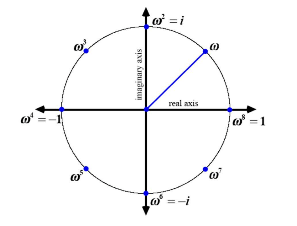
A complex number \(\omega\) is an \(n^{\text {th }}\) root of unity if it satisfies \(\omega^n=1\).
There are exactly \(n\) complex \(n^{\text {th }}\) roots of unity, which can be written as
\(e^{\frac{2 \pi i k}{n}}, \quad k=0,1, \ldots, n-1.\)
Observe the useful fact that
\(e^{\frac{2 \pi i k}{n}}=\left(e^{\frac{2 \pi i}{n}}\right)^k,\)
i.e., the roots of unity can all be defined as powers of the \(k=1^{\text {st }}\) one.
We call the first one a primitive \(n^{\text {th }}\) root of unity.
More specifically, \(\omega\) is a primitive \(n^{\text {th }}\) root of unity if:
\(\begin{aligned}& \omega^n=1 \\& \omega^j \neq 1 \quad \text { for } 0<j<n\end{aligned}\)
(Youtube)
(Desmos)
Discrete Fourier Transform
For \(A\), a polynomial of degree \(N-1\) expressed in coeffiecent form:
\(A(x)=a_0+a_1 x+a_2 x_2+\cdots+a_{N-1} x^{N-1},\)
define the DFT (Discrete Fourier Transform) of the coefficient vector \(\left(a_0, \ldots, a_{N-1}\right)\) to be another vector of \(N\) numbers as follows:
\(F_N\left(a_0, a_1, \ldots, a_{N-1}\right)=\left(A\left(\omega^0\right), A\left(\omega^1\right), \ldots, A\left(\omega^{N-1}\right)\right),\)
where \(\omega\) is a \(N^{th}\) root of unity.
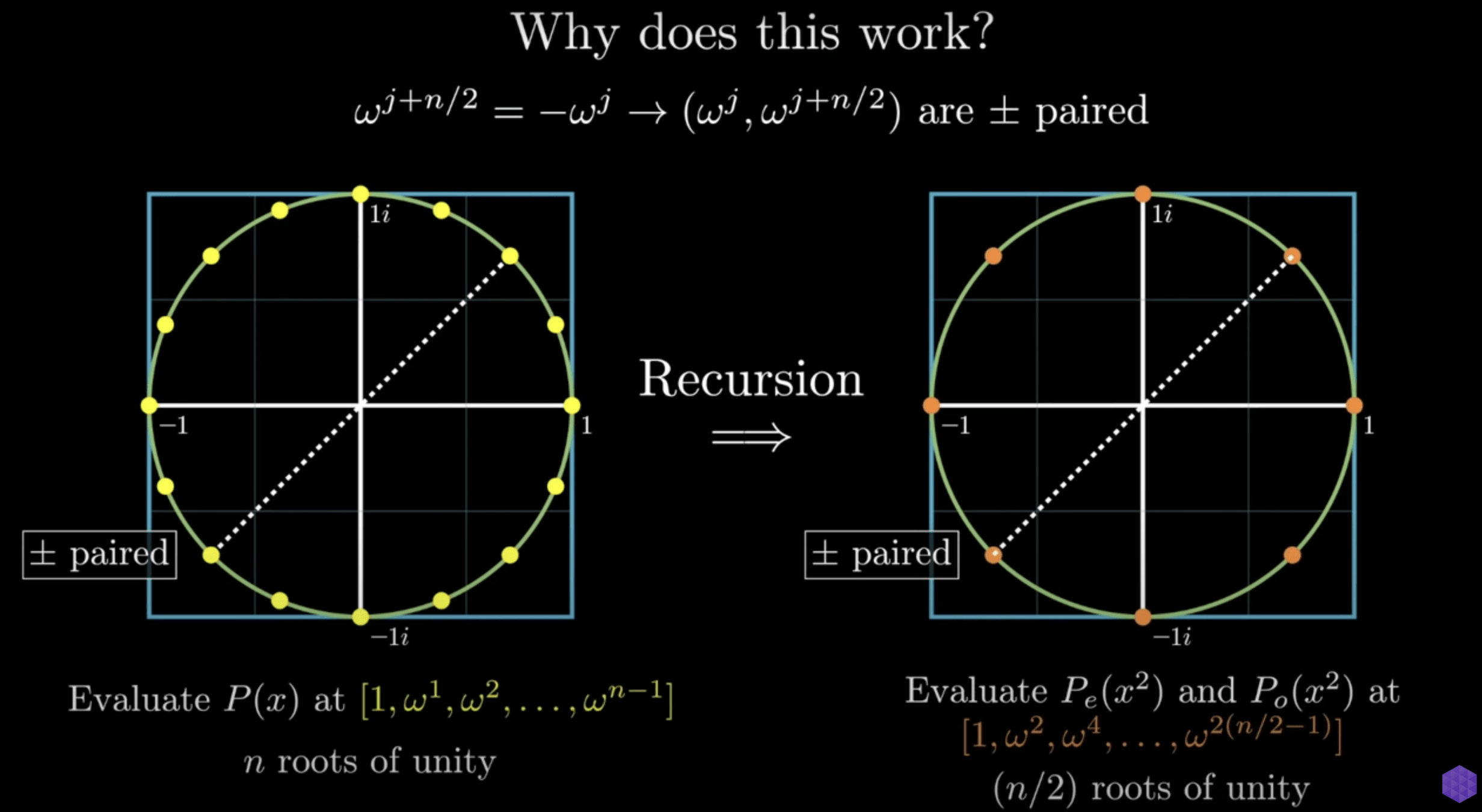
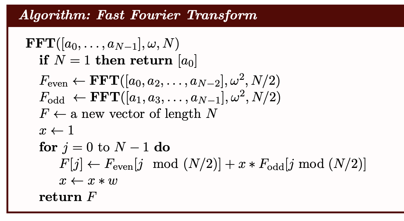
Fast Fourier Transform
\(F_N(A)_j = A\left(\omega^j\right)\)
\(=\sum_{i=0}^{N-1} a_i \omega^{i j}\)
\(=\sum_{i=0}^{\frac{N}{2}-1} a_{2 i} \omega^{2 i j}+\sum_{i=0}^{\frac{N}{2}-1} a_{2 i+1} \omega^{(2 i+1) j}\)
\(=\sum_{i=0}^{N-1} a_i \omega^{i j}+\sum_{i=1}^{N-1} a_i \omega^{i j}\)
i even
i odd
\(= \sum_{i=0}^{\frac{N}{2}-1} a_{2 i}\left(\omega^2\right)^{i j}+\omega^j \sum_{i=0}^{\frac{N}{2}-1} a_{2 i+1}\left(\omega^2\right)^{i j}\)
\(= \sum_{i=0}^{\frac{N}{2}-1} a_{2 i}\left(\omega_{N / 2}\right)^{i(j \bmod N / 2)}+\omega_N^j \sum_{i=0}^{\frac{N}{2}-1} a_{2 i+1}\left(\omega_{N / 2}\right)^{i(j \bmod N / 2)}\)
Fast Fourier Transform
(Source)
\(F_N(A)_j=F_{N / 2}\left({\color{IndianRed}A_{\text {even }}}\right)_{j \bmod N / 2}+\omega_N^j F_{N / 2}\left({\color{DodgerBlue}A_{\text {odd }}}\right)_{j \bmod N / 2}\)
The Inverse of the DFT
\(\left(\begin{array}{cccc}\omega^{0 \cdot 0} & \omega^{0 \cdot 1} & \cdots & \omega^{0 \cdot(N-1)} \\ \omega^{1 \cdot 0} & \omega^{1 \cdot 1} & \cdots & \omega^{1 \cdot(N-1)} \\ \vdots & \vdots & \ddots & \vdots \\ \omega^{(N-1) \cdot 0} & \omega^{(N-1) \cdot 1} & \cdots & \omega^{(N-1) \cdot(N-1)}\end{array}\right)\left(\begin{array}{c}a_0 \\ a_1 \\ \vdots \\ a_{N-1}\end{array}\right)\)
\(= \left(A\left(\omega^0\right), A\left(\omega^1\right), \ldots, A\left(\omega^{N-1}\right)\right)^T\)
Let's call this matrix DFT \((\omega, N)\).
What we need is \(\operatorname{DFT}(\omega, N)^{-1}\).
The Inverse of the DFT
The \((k, j)\) entry of \(\mathbf{D F T}\left(\omega^{-1}, N\right) \mathbf{D F T}(\omega, N)= \begin{cases}N & \text { if } k=j \\ 0 & \text { if } k \neq j\end{cases}\)
\(\boldsymbol{\operatorname { D F T }}(\omega, N)^{-1}=\frac{1}{N} \boldsymbol{\operatorname { D F T }}\left(\omega^{-1}, N\right)\)
Exercise:
\(\mathbf{D F T}\left(\omega^{-1}, N\right) \mathbf{D F T}(\omega, N)= N \cdot I_n \)
Polynomial Multiplication
\(A(x)=a_0 x^0+a_1 x^1+\cdots+a_{n-1} x^{n-1}\)
\(B(x)=b_0 x^0+b_1 x^1+\cdots+b_{m-1} x^{m-1}\)
\(C = A\cdot B\)
\(+ 0x_{n+1} + \cdots + 0x_{n+m-1}\).
\({\color{IndianRed}A := \{a_0,\ldots,a_{n-1}\}},{\color{DodgerBlue}B := \{b_0, \ldots, b_{m-1}\}}\)
\(+ 0x_{m+1} + \cdots + 0x_{n+m-1}\).
\({\color{IndianRed}(0,A(0)),\ldots,(n+m-1,A(n+m-1))},\\{\color{DodgerBlue}(0,B(0)),\ldots,(n+m-1,B(n+m-1))}\)
\({\color{SeaGreen}(0,C(0)),\ldots,(n+m-1,C(m+n-1))}\)
\({\color{SeaGreen}c_0,\ldots,c_{m+n-1}}\)
FFT
Inv
FFT
Advanced Algorithms
Part 2. Fast Fourier Transforms
Part 1a. Polynomial Multiplication, DFT, and FFT
Part 1b. Variations of FFT
Part 1c. Examples and Applications
Part 1d. DP Speedup: Counting Road Networks
Part 1e. DP Speedup: Tiles
Advanced Algorithms
Part 2. Fast Fourier Transforms
Part 1a. Polynomial Multiplication, DFT, and FFT
Part 1b. Variations of FFT
Part 1c. Examples and Applications
Part 1d. DP Speedup: Counting Road Networks
Part 1e. DP Speedup: Tiles
Advanced Algorithms
Part 2. Fast Fourier Transforms
Part 1a. Polynomial Multiplication, DFT, and FFT
Part 1b. Variations of FFT
Part 1c. Examples and Applications
Part 1d. DP Speedup: Counting Road Networks
Part 1e. DP Speedup: Tiles
Counting Road Networks
Lukas is a Civil Engineer who loves designing road networks to connect \(\boldsymbol{n}\) cities numbered from 1 to \(\boldsymbol{n}\).
He can build any number of bidirectional roads as long as the resultant network satisfies these constraints:
1. It must be possible to reach any city from any other city by traveling along the network of roads.
2. No two roads can directly connect the same two cities.
3. A road cannot directly connect a city to itself.
In other words, the roads and cities must form a simple connected labeled graph.
You must answer \(q\) queries, where each query consists of some \(\boldsymbol{n}\) denoting the number of cities Lukas wants to design a bidirectional network of roads for. For each query, find the number of ways he can build roads connecting \(n\) cities.
Counting Road Networks
How many connected graphs are there on \(n\) vertices?
Let \(f(n)\) be the answer for \(n\).
To compute \(f(n)\), we
subtract the number of disconnected graphs from the total number.
The total number of size- \(n\) graphs is \(g(n):=2^{\binom{n}{2}}\).
How to count the disconnected graphs?
Counting Road Networks
Let's consider the size \(m\) of the connected component
containing the vertex labeled with 1 .
Since the graph is disconnected, \(m\) cannot be \(n\).
Then the number of disconnected graphs where the connected component containing vertex 1 has size \(m\) is exactly:
\(f(m) \cdot g(n-m)\)
Counting Road Networks
\(f(n)={\color{SeaGreen}g(n)}-\sum_{m=1}^{n-1}\binom{n-1}{m-1} \cdot f(m) \cdot g(n-m)\)
If we unfold the binomial coefficients, we will have
Let \(F(n):=\frac{f(n)}{(n-1)!}\) and \(G(n):=\frac{g(n)}{n!}\).
If we set \(F(0)\) to 0, then we have:
\(F(n)=n \cdot G(n)-\sum_{m=0}^{n-1} F(m) \cdot G(n-m)\)
\(\frac{f(n)}{{\color{IndianRed}(n-1)!}}= {\color{IndianRed}n} \cdot \frac{g(n)}{{\color{IndianRed}n!}}-\sum_{m=1}^{n-1} \frac{f(m)}{{\color{IndianRed}(m-1)!}} \cdot \frac{g(n-m)}{{\color{IndianRed}(n-m)!}}\)
Counting Road Networks
\(F(n)=n \cdot G(n)-\sum_{m=0}^{n-1} F(m) \cdot G(n-m)\)
\(G(n)\) are easy to compute so we can pre-process them.
Let solve \((\ell, r)\) be a procedure that computes \(F(n)\) for all \(n \in[l, r)\).
Invariant: When invoking solve \((\ell, r)\), we have computed for each \(n \in[\ell, r)\), the partial convolution \(\sum_{m=0}^{\ell-1} F(m) \cdot G(n-m)\), and store them in \(H(n)\).
In general, move from solve\((\ell,r)\) to
solve\((\ell,k)\) & solve\((k,r)\),
where \(k := \frac{\ell+r}{2}\).
Counting Road Networks
\(F(n)=n \cdot G(n)-\sum_{m=0}^{n-1} F(m) \cdot G(n-m)\)
Invariant: When invoking solve \((\ell, r)\), we have computed for each \(n \in[\ell, r)\), the partial convolution \(\sum_{m=0}^{\ell-1} F(m) \cdot G(n-m)\), and store them in \(H(n)\).
1
9
5
In general, move from solve\((\ell,r)\) to
solve\((\ell,k)\) & solve\((k,r)\),
where \(k := \frac{\ell+r}{2}\).
Counting Road Networks
\(F(n)=n \cdot G(n)-\sum_{m=0}^{n-1} F(m) \cdot G(n-m)\)
Invariant: When invoking solve \((\ell, r)\), we have computed for each \(n \in[\ell, r)\), the partial convolution \(\sum_{m=0}^{\ell-1} F(m) \cdot G(n-m)\), and store them in \(H(n)\).
\(H(n) \leftarrow H(n)+\sum_{m=\ell}^{k-1} F(m) \cdot G(n-m)\)
In general, move from solve\((\ell,r)\) to
solve\((\ell,k)\) & solve\((k,r)\),
where \(k := \frac{\ell+r}{2}\).
Counting Road Networks
\(F(n)=n \cdot G(n)-\sum_{m=0}^{n-1} F(m) \cdot G(n-m)\)
In general, move from solve\((\ell,r)\) to
solve\((\ell,k)\) & solve\((k,r)\),
where \(k := \frac{\ell+r}{2}\).
Invariant: When invoking solve \((\ell, r)\), we have computed for each \(n \in[\ell, r)\), the partial convolution \(\sum_{m=0}^{\ell-1} F(m) \cdot G(n-m)\), and store them in \(H(n)\).
\(H(n) \leftarrow H(n)+\underbrace{\sum_{m=\ell}^{k-1} F(m) \cdot G(n-m)}_{\text{convolution}}\)
Counting Road Networks
\(F(n)=n \cdot G(n)-\sum_{m=0}^{n-1} F(m) \cdot G(n-m)\)
In general, move from solve\((\ell,r)\) to
solve\((\ell,k)\) & solve\((k,r)\),
where \(k := \frac{\ell+r}{2}\).
Invariant: When invoking solve \((\ell, r)\), we have computed for each \(n \in[\ell, r)\), the partial convolution \(\sum_{m=0}^{\ell-1} F(m) \cdot G(n-m)\), and store them in \(H(n)\).
\(C(n)=\sum_{m=\ell}^{k-1} F(m) \cdot G(n-m)\)
Use FFT to compute this in \(O(q \log q)\) time, where \(q\) is the number of summands.
Counting Road Networks
\(F(n)=n \cdot G(n)-\sum_{m=0}^{n-1} F(m) \cdot G(n-m)\)
In general, move from solve\((\ell,r)\) to
solve\((\ell,k)\) & solve\((k,r)\),
where \(k := \frac{\ell+r}{2}\).
Invariant: When invoking solve \((\ell, r)\), we have computed for each \(n \in[\ell, r)\), the partial convolution \(\sum_{m=0}^{\ell-1} F(m) \cdot G(n-m)\), and store them in \(H(n)\).
Base Case
If \(\ell+1=r\), we set \(F(\ell)\) to \(\ell \cdot G(\ell)-H(\ell)\).
Advanced Algorithms
Part 2. Fast Fourier Transforms
Part 1a. Polynomial Multiplication, DFT, and FFT
Part 1b. Variations of FFT
Part 1c. Examples and Applications
Part 1d. DP Speedup: Counting Road Networks
Part 1e. DP Speedup: Tiles
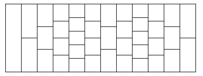
Tiles
(source)
Tiles
(source)
The road is constructed as follows:
- the first row consists of 1 tile;
- then \(a_1\) rows follow; each of these rows contains 1 tile greater than the previous row;
- then \(b_1\) rows follow; each of these rows contains 1 tile less than the previous row;
- then \(a_2\) rows follow; each of these rows contains 1 tile greater than the previous row;
- then \(b_2\) rows follow; each of these rows contains 1 tile less than the previous row;
\(\vdots\)
- then \(a_n\) rows follow; each of these rows contains 1 tile greater than the previous row;
- then \(b_n\) rows follow; each of these rows contains 1 tile less than the previous row.
Tiles
(source)
Calculate the number of different paths from the first row to the last row.
AdvAlgo 02
By Neeldhara Misra


