Parameterized Approaches
Neeldhara Misra
to
KEMENY RANK AGGREGATION
IISc MSR Seminar Series
18 FEB 2022
(CSE @IIT Gandhinagar)
Plan
Input.
A collection of rankings
over a set of alternatives.
Input.
A collection of rankings
over a set of alternatives.
Input.
A collection of partial orders
over a set of alternatives.
Input.
A collection of weak orders
over a set of alternatives.
Input.
A collection of rankings
over a set of alternatives.
Input.
A collection of rankings
over a set of alternatives.
Output.
A single consensus ranking.
Input.
A collection of rankings
over a set of alternatives.
Output.
A single consensus ranking.
🍕 \(\succ\) 🍔 \(\succ\) 🍰 \(\succ\) 🍩 \(\succ\) 🌮
🍰 \(\succ\) 🍕 \(\succ\) 🌮 \(\succ\) 🍩 \(\succ\) 🍔
🍰 \(\succ\) 🍕 \(\succ\) 🍔 \(\succ\) 🍩 \(\succ\) 🌮
🌮 \(\succ\) 🍔 \(\succ\) 🍰 \(\succ\) 🍩 \(\succ\) 🍕
🌮 \(\succ\) 🍰 \(\succ\) 🍕 \(\succ\) 🍩 \(\succ\) 🍔
🍕 \(\succ\) 🍔 \(\succ\) 🍰 \(\succ\) 🍩 \(\succ\) 🌮
🍰 \(\succ\) 🍕 \(\succ\) 🌮 \(\succ\) 🍩 \(\succ\) 🍔
🍰 \(\succ\) 🍕 \(\succ\) 🍔 \(\succ\) 🍩 \(\succ\) 🌮
🌮 \(\succ\) 🍔 \(\succ\) 🍰 \(\succ\) 🍩 \(\succ\) 🍕
🌮 \(\succ\) 🍰 \(\succ\) 🍕 \(\succ\) 🍩 \(\succ\) 🍔
Input.
A collection of rankings
over a set of alternatives.
Output.
A single consensus ranking.
Input.
A collection of rankings
over a set of alternatives.
Output.
A single ranking that satisfies unanimity, yada yada.
Input.
A collection of rankings
over a set of alternatives.
Output.
A single ranking that satisfies unanimity, yada yada.
Input.
A collection of rankings
over a set of alternatives.
Output.
A single ranking that minimises
dissatisfication.
🍕 \(\succ\) 🍔 \(\succ\) 🍰 \(\succ\) 🍩 \(\succ\) 🌮
🍰 \(\succ\) 🍕 \(\succ\) 🌮 \(\succ\) 🍩 \(\succ\) 🍔
🍰 \(\succ\) 🍕 \(\succ\) 🍔 \(\succ\) 🍩 \(\succ\) 🌮
🌮 \(\succ\) 🍔 \(\succ\) 🍰 \(\succ\) 🍩 \(\succ\) 🍕
🌮 \(\succ\) 🍰 \(\succ\) 🍕 \(\succ\) 🍩 \(\succ\) 🍔
🍕 \(\succ\) 🍔 \(\succ\) 🍰 \(\succ\) 🍩 \(\succ\) 🌮
🍰 \(\succ\) 🍕 \(\succ\) 🌮 \(\succ\) 🍩 \(\succ\) 🍔
🍰 \(\succ\) 🍕 \(\succ\) 🍔 \(\succ\) 🍩 \(\succ\) 🌮
🌮 \(\succ\) 🍔 \(\succ\) 🍰 \(\succ\) 🍩 \(\succ\) 🍕
🌮 \(\succ\) 🍰 \(\succ\) 🍕 \(\succ\) 🍩 \(\succ\) 🍔
🍰 \(\succ\) 🍕 \(\succ\) 🍔 \(\succ\) 🍩 \(\succ\) 🌮
🍕 \(\succ\) 🍔 \(\succ\) 🍰 \(\succ\) 🍩 \(\succ\) 🌮
🍰 \(\succ\) 🍕 \(\succ\) 🍔 \(\succ\) 🍩 \(\succ\) 🌮
v/s
🍰 \(\succ\) 🍕 \(\succ\) 🌮 \(\succ\) 🍩 \(\succ\) 🍔
🍰 \(\succ\) 🍕 \(\succ\) 🍔 \(\succ\) 🍩 \(\succ\) 🌮
v/s
🍰 \(\succ\) 🍕 \(\succ\) 🍔 \(\succ\) 🍩 \(\succ\) 🌮
🍰 \(\succ\) 🍕 \(\succ\) 🍔 \(\succ\) 🍩 \(\succ\) 🌮
v/s
🌮 \(\succ\) 🍔 \(\succ\) 🍰 \(\succ\) 🍩 \(\succ\) 🍕
🍰 \(\succ\) 🍕 \(\succ\) 🍔 \(\succ\) 🍩 \(\succ\) 🌮
v/s
🌮 \(\succ\) 🍰 \(\succ\) 🍕 \(\succ\) 🍩 \(\succ\) 🍔
🍰 \(\succ\) 🍕 \(\succ\) 🍔 \(\succ\) 🍩 \(\succ\) 🌮
v/s
🌮 \(\succ\) 🍰 \(\succ\) 🍕 \(\succ\) 🍩 \(\succ\) 🍔
🍰 \(\succ\) 🍕 \(\succ\) 🍔 \(\succ\) 🍩 \(\succ\) 🌮
A notion of distance
between permutations would be
a useful measure of dissatisfaction.
🌮 \(\succ\) 🍰 \(\succ\) 🍕 \(\succ\) 🍩 \(\succ\) 🍔
🍰 \(\succ\) 🍕 \(\succ\) 🍔 \(\succ\) 🍩 \(\succ\) 🌮
| 🍰 | 🍕 | 🍔 | 🍩 | 🌮 | |
|---|---|---|---|---|---|
| 🍰 | |||||
| 🍕 | |||||
| 🍔 | |||||
| 🍩 | |||||
| 🌮 |
🌮 \(\succ\) 🍰 \(\succ\) 🍕 \(\succ\) 🍩 \(\succ\) 🍔
🍰 \(\succ\) 🍕 \(\succ\) 🍔 \(\succ\) 🍩 \(\succ\) 🌮
| 🍰 | 🍕 | 🍔 | 🍩 | 🌮 | |
|---|---|---|---|---|---|
| 🍰 | ✔️ | ||||
| 🍕 | |||||
| 🍔 | |||||
| 🍩 | |||||
| 🌮 |
🌮 \(\succ\) 🍰 \(\succ\) 🍕 \(\succ\) 🍩 \(\succ\) 🍔
🍰 \(\succ\) 🍕 \(\succ\) 🍔 \(\succ\) 🍩 \(\succ\) 🌮
| 🍰 | 🍕 | 🍔 | 🍩 | 🌮 | |
|---|---|---|---|---|---|
| 🍰 | ✔️ | ✔️ | |||
| 🍕 | |||||
| 🍔 | |||||
| 🍩 | |||||
| 🌮 |
🌮 \(\succ\) 🍰 \(\succ\) 🍕 \(\succ\) 🍩 \(\succ\) 🍔
🍰 \(\succ\) 🍕 \(\succ\) 🍔 \(\succ\) 🍩 \(\succ\) 🌮
| 🍰 | 🍕 | 🍔 | 🍩 | 🌮 | |
|---|---|---|---|---|---|
| 🍰 | ✔️ | ✔️ | ✔️ | ||
| 🍕 | |||||
| 🍔 | |||||
| 🍩 | |||||
| 🌮 |
🌮 \(\succ\) 🍰 \(\succ\) 🍕 \(\succ\) 🍩 \(\succ\) 🍔
🍰 \(\succ\) 🍕 \(\succ\) 🍔 \(\succ\) 🍩 \(\succ\) 🌮
| 🍰 | 🍕 | 🍔 | 🍩 | 🌮 | |
|---|---|---|---|---|---|
| 🍰 | ✔️ | ✔️ | ✔️ | 🤦♀️ | |
| 🍕 | |||||
| 🍔 | |||||
| 🍩 | |||||
| 🌮 |
🌮 \(\succ\) 🍰 \(\succ\) 🍕 \(\succ\) 🍩 \(\succ\) 🍔
🍰 \(\succ\) 🍕 \(\succ\) 🍔 \(\succ\) 🍩 \(\succ\) 🌮
| 🍰 | 🍕 | 🍔 | 🍩 | 🌮 | |
|---|---|---|---|---|---|
| 🍰 | ✔️ | ✔️ | ✔️ | 🤦♀️ | |
| 🍕 | ✔️ | ||||
| 🍔 | |||||
| 🍩 | |||||
| 🌮 |
🌮 \(\succ\) 🍰 \(\succ\) 🍕 \(\succ\) 🍩 \(\succ\) 🍔
🍰 \(\succ\) 🍕 \(\succ\) 🍔 \(\succ\) 🍩 \(\succ\) 🌮
| 🍰 | 🍕 | 🍔 | 🍩 | 🌮 | |
|---|---|---|---|---|---|
| 🍰 | ✔️ | ✔️ | ✔️ | 🤦♀️ | |
| 🍕 | ✔️ | ✔️ | |||
| 🍔 | |||||
| 🍩 | |||||
| 🌮 |
🌮 \(\succ\) 🍰 \(\succ\) 🍕 \(\succ\) 🍩 \(\succ\) 🍔
🍰 \(\succ\) 🍕 \(\succ\) 🍔 \(\succ\) 🍩 \(\succ\) 🌮
| 🍰 | 🍕 | 🍔 | 🍩 | 🌮 | |
|---|---|---|---|---|---|
| 🍰 | ✔️ | ✔️ | ✔️ | 🤦♀️ | |
| 🍕 | ✔️ | ✔️ | 🤷♀️ | ||
| 🍔 | |||||
| 🍩 | |||||
| 🌮 |
🌮 \(\succ\) 🍰 \(\succ\) 🍕 \(\succ\) 🍩 \(\succ\) 🍔
🍰 \(\succ\) 🍕 \(\succ\) 🍔 \(\succ\) 🍩 \(\succ\) 🌮
| 🍰 | 🍕 | 🍔 | 🍩 | 🌮 | |
|---|---|---|---|---|---|
| 🍰 | ✔️ | ✔️ | ✔️ | 🤦♀️ | |
| 🍕 | ✔️ | ✔️ | 🤷♀️ | ||
| 🍔 | 😡 | ||||
| 🍩 | |||||
| 🌮 |
🌮 \(\succ\) 🍰 \(\succ\) 🍕 \(\succ\) 🍩 \(\succ\) 🍔
🍰 \(\succ\) 🍕 \(\succ\) 🍔 \(\succ\) 🍩 \(\succ\) 🌮
| 🍰 | 🍕 | 🍔 | 🍩 | 🌮 | |
|---|---|---|---|---|---|
| 🍰 | ✔️ | ✔️ | ✔️ | 🤦♀️ | |
| 🍕 | ✔️ | ✔️ | 🤷♀️ | ||
| 🍔 | 😡 | 🥺 | |||
| 🍩 | |||||
| 🌮 |
🌮 \(\succ\) 🍰 \(\succ\) 🍕 \(\succ\) 🍩 \(\succ\) 🍔
🍰 \(\succ\) 🍕 \(\succ\) 🍔 \(\succ\) 🍩 \(\succ\) 🌮
| 🍰 | 🍕 | 🍔 | 🍩 | 🌮 | |
|---|---|---|---|---|---|
| 🍰 | ✔️ | ✔️ | ✔️ | 🤦♀️ | |
| 🍕 | ✔️ | ✔️ | 🤷♀️ | ||
| 🍔 | 😡 | 🥺 | |||
| 🍩 | 😭 | ||||
| 🌮 |
distance = #of disagreements
Input.
A collection of rankings
over a set of alternatives.
Output.
A single ranking that minimises
the total Kendall tau or bubble sort distance.

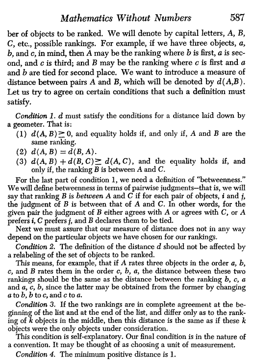
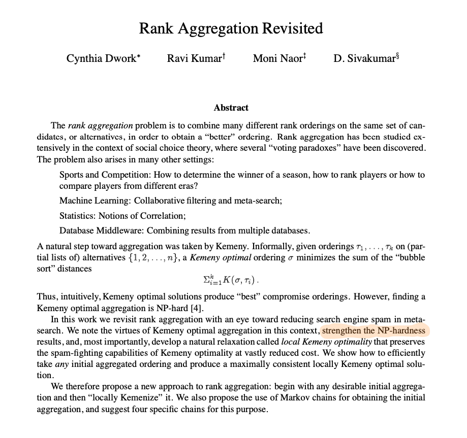
Bartholdi, Tovey and Tick, Social Choice and Welfare 1989,
Dwork, Kumar, Naor, and Sivakumar, WWW 2001
The problem of computing
a Kemeny optimal permutation
for a given collection of \(k\) full lists, for even integers \(k \geq 4\),
is NP-hard.
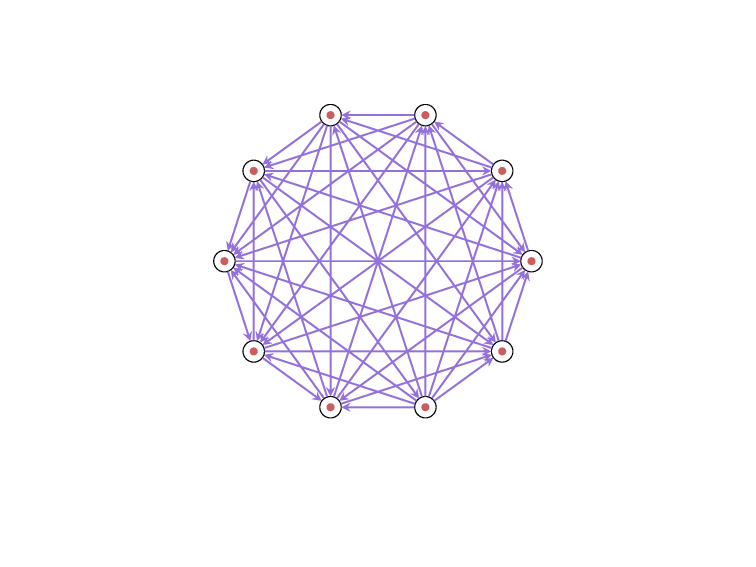
Minimum Feedback Edge Set
Minimum Feedback Edge Set
on Directed Graphs
Minimum Feedback Edge Set
on Directed Graphs
Minimum Feedback Edge Set
on Directed Graphs
Minimum Feedback Edge Set
on Directed Graphs
Minimum Feedback Edge Set
on Directed Graphs
Minimum Feedback Edge Set
on Directed Graphs
Minimum Feedback Edge Set
on Directed Graphs
Minimum Feedback Edge Set
on Directed Graphs
1
2
3
4
5
6
7
8
a
b
c
d
e
f
g
h
i
Minimum Feedback Edge Set
on Directed Graphs
1
2
3
4
5
6
7
8
a
b
c
d
e
f
g
h
i
1
Minimum Feedback Edge Set
on Directed Graphs
1
2
3
4
5
6
7
8
a
b
c
d
e
f
g
h
i
1
2
a
Minimum Feedback Edge Set
on Directed Graphs
1
2
3
4
5
6
7
8
a
b
c
d
e
f
g
h
i
1
2
a
3
b
d
Minimum Feedback Edge Set
on Directed Graphs
1
2
3
4
5
6
7
8
a
b
c
d
e
f
g
h
i
1
2
a
3
b
d
4
c
f
Minimum Feedback Edge Set
on Directed Graphs
1
2
3
4
5
6
7
8
a
b
c
d
e
f
g
h
i
1
2
a
3
b
d
4
c
f
5
g
Minimum Feedback Edge Set
on Directed Graphs
1
2
3
4
5
6
7
8
a
b
c
d
e
f
g
h
i
1
2
a
3
b
d
4
c
f
5
g
6
e
Minimum Feedback Edge Set
on Directed Graphs
1
2
3
4
5
6
7
8
a
b
c
d
e
f
g
h
i
1
2
a
3
b
d
4
c
f
5
g
6
e
7
h
Minimum Feedback Edge Set
on Directed Graphs
1
2
3
4
5
6
7
8
a
b
c
d
e
f
g
h
i
1
2
a
3
b
d
4
c
f
5
g
6
e
7
h
8
i
Minimum Feedback Edge Set
on Directed Graphs
1
2
3
4
5
6
7
8
a
b
c
d
e
f
g
h
i
Minimum Feedback Edge Set
on Directed Graphs
1
2
3
4
5
6
7
8
a
b
c
d
e
f
g
h
i
1
a
b
Minimum Feedback Edge Set
on Directed Graphs
1
2
3
4
5
6
7
8
a
b
c
d
e
f
g
h
i
2
c
1
a
b
Minimum Feedback Edge Set
on Directed Graphs
1
2
3
4
5
6
7
8
a
b
c
d
e
f
g
h
i
3
e
2
c
1
a
b
Minimum Feedback Edge Set
on Directed Graphs
1
2
3
4
5
6
7
8
a
b
c
d
e
f
g
h
i
d
4
3
e
2
c
1
a
b
Minimum Feedback Edge Set
on Directed Graphs
1
2
3
4
5
6
7
8
a
b
c
d
e
f
g
h
i
f
5
i
d
4
3
e
2
c
1
a
b
Minimum Feedback Edge Set
on Directed Graphs
1
2
3
4
5
6
7
8
a
b
c
d
e
f
g
h
i
g
6
f
5
i
d
4
3
e
2
c
1
a
b
h
Minimum Feedback Edge Set
on Directed Graphs
1
2
3
4
5
6
7
8
a
b
c
d
e
f
g
h
i
g
6
f
5
i
d
4
3
e
2
c
1
a
b
h
7
Minimum Feedback Edge Set
on Directed Graphs
1
2
3
4
5
6
7
8
a
b
c
d
e
f
g
h
i
g
6
f
5
i
d
4
3
e
2
c
1
a
b
h
7
8
Minimum Feedback Edge Set
on Directed Graphs
1
2
3
4
5
6
7
8
a
b
c
d
e
f
g
h
i
g
f
i
d
e
c
h
a
b
d
c
f
g
e
h
i
a
b
1
2
3
4
5
6
7
8
1
2
3
4
5
6
7
8
Minimum Feedback Edge Set
on Directed Graphs
1
2
3
4
5
6
7
8
a
b
d
e
g
h
i
g
i
d
e
h
a
b
d
g
e
h
i
a
b
1
2
3
4
5
6
7
8
1
2
3
4
5
6
7
8
f
f
c
c
c
f
Minimum Feedback Edge Set
on Directed Graphs
1
2
3
4
5
6
7
8
a
b
d
e
g
h
i
g
i
d
e
h
a
b
d
g
e
h
i
a
b
1
2
3
4
5
6
7
8
1
2
3
4
5
6
7
8
f
f
c
c
c
f
1
2
3
4
5
6
7
8
a
b
d
e
g
h
i
g
i
d
e
h
a
b
d
g
e
h
i
a
b
1
2
3
4
5
6
7
8
1
2
3
4
5
6
7
8
f
f
c
c
c
f
g
i
e
h
a
g
e
h
i
a
b
8
7
6
5
4
3
2
1
f
f
c
c
b
d
8
7
6
5
4
3
2
1
d
If two rankings \(\sigma\) and \(\tau\)
are complete opposites,
then any ranking \(\rho\) will have
a total Kemeny distance of \({n \choose 2}\)
from both of them combined.
1
2
3
4
5
6
7
8
7
6
5
4
3
2
1
8
1
2
3
4
5
6
7
8
8
7
6
5
4
3
2
1
1
2
3
4
5
6
7
8
8
7
6
5
4
3
2
1
7
3
1
2
3
4
5
6
7
8
8
6
5
4
2
1
7
3
7
3
1
2
4
5
6
8
8
6
5
4
2
1
7
3
7
3
3
7
This creates a neat
cancelation effect
& forces a minimum Kemeny score of
\(2{n \choose 2} + 2{m \choose 2} + 2m\)
on any ranking.
1
2
3
4
5
6
7
8
a
b
d
e
g
h
i
g
i
d
e
h
a
b
d
g
e
h
i
a
b
1
2
3
4
5
6
7
8
1
2
3
4
5
6
7
8
f
f
c
c
c
f
g
i
e
h
a
g
e
h
i
a
b
8
7
6
5
4
3
2
1
f
f
c
c
b
d
8
7
6
5
4
3
2
1
d
This creates a neat
cancelation effect
& forces a minimum Kemeny score of
\(2{n \choose 2} + 2{m \choose 2} + 2m\)
on any ranking.
This creates a neat
cancelation effect
& forces a minimum Kemeny score of
\(2{n \choose 2} + 2{m \choose 2} + 2m\)
on any ranking.
+ 2k
if and only if G has a FES of size at most k.
final score \(\leq\)
(The cost of the backedges can be isolated.)
factor 11/7-approximation (randomised):
Ailon, Charikar, and Newman, STOC 2005 → JACM 2008
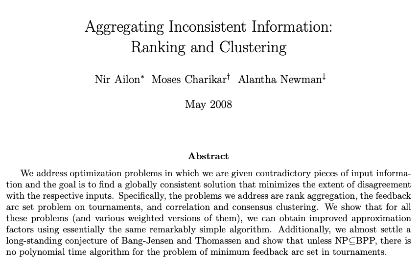
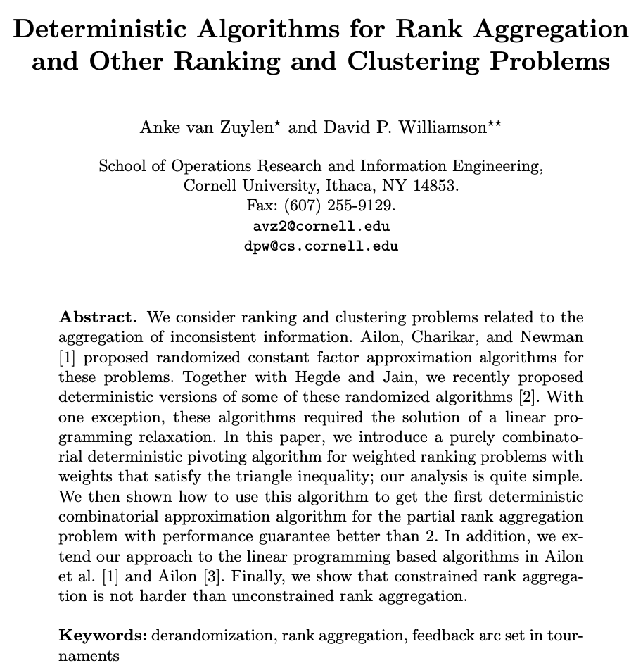
factor 8/5-approximation:
van Zuylen and Williamson, WAOA 2007
Kenyon-Mathieu and Schudy, STOC 2007
Parameterized
Approaches
🤨
FPT Algorithm:
Solve the problem in time \(f(k)\cdot n^{O(1)}\), for some appropriate parameter \(k\).
Kernelization:
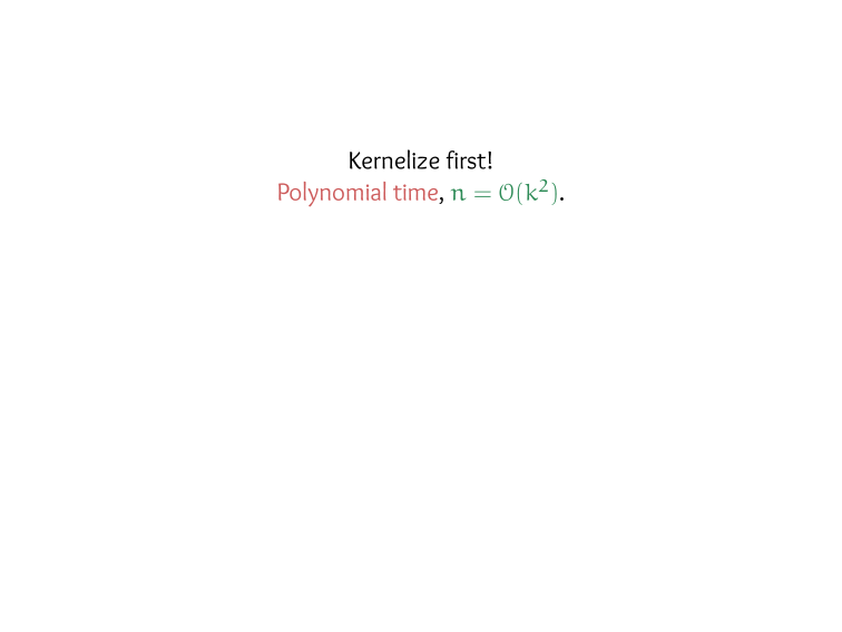
Reduce the problem in time \(n^{O(1)}\),
to an equivalent instance whose size is bounded by \(f(k)\),
for some appropriate parameter \(k\).
- number of votes \(n\)
- number of candidates \(m\)
- Kemeny score \(k\)
- max. range of candidate positions
- avg. range of candidate positions
- avg. KT-distance \(d_a\)
- max. KT-distance \(d_m\)
- number of votes \(n\)
- number of candidates \(m\)
- Kemeny score \(k\)
- max. range of candidate positions
- avg. range of candidate positions
- avg. KT-distance \(d_a\)
- max. KT-distance \(d_m\)
Marek Karpinski and Warren Schudy; ISAAC 2010
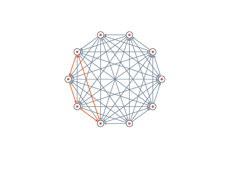

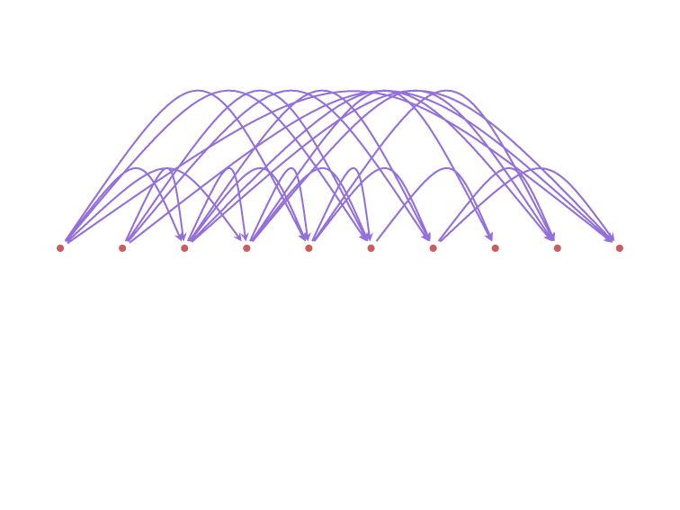

🍕 \(\succ\) 🍔 \(\succ\) 🍰 \(\succ\) 🍩 \(\succ\) 🌮
🍰 \(\succ\) 🍕 \(\succ\) 🌮 \(\succ\) 🍩 \(\succ\) 🍔
🍰 \(\succ\) 🍕 \(\succ\) 🍔 \(\succ\) 🍩 \(\succ\) 🌮
🌮 \(\succ\) 🍔 \(\succ\) 🍰 \(\succ\) 🍩 \(\succ\) 🍕
🌮 \(\succ\) 🍰 \(\succ\) 🍕 \(\succ\) 🍩 \(\succ\) 🍔
🍕 \(\succ\) 🍔 \(\succ\) 🍰 \(\succ\) 🍩 \(\succ\) 🌮
🍰 \(\succ\) 🍕 \(\succ\) 🌮 \(\succ\) 🍩 \(\succ\) 🍔
🍰 \(\succ\) 🍕 \(\succ\) 🍔 \(\succ\) 🍩 \(\succ\) 🌮
🌮 \(\succ\) 🍔 \(\succ\) 🍰 \(\succ\) 🍩 \(\succ\) 🍕
🌮 \(\succ\) 🍰 \(\succ\) 🍕 \(\succ\) 🍩 \(\succ\) 🍔
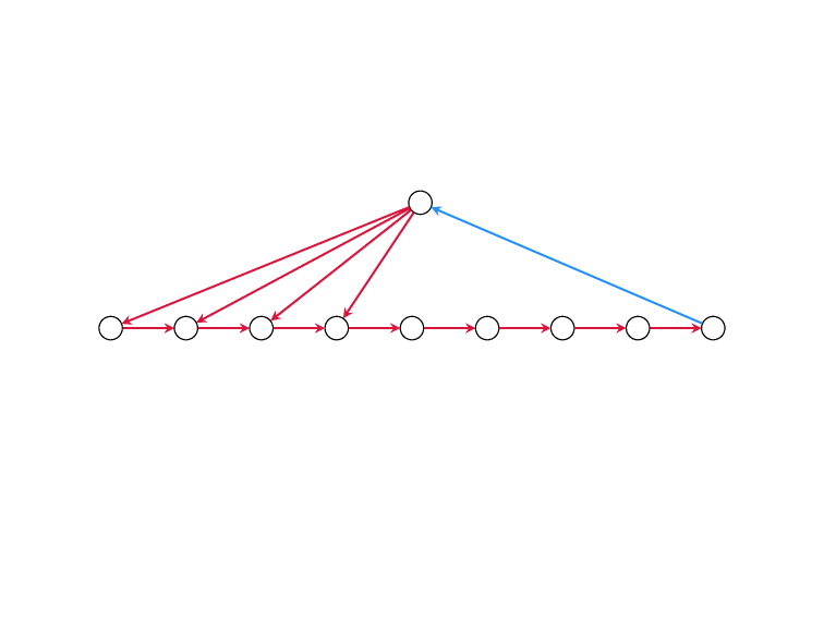
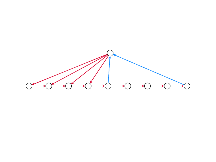
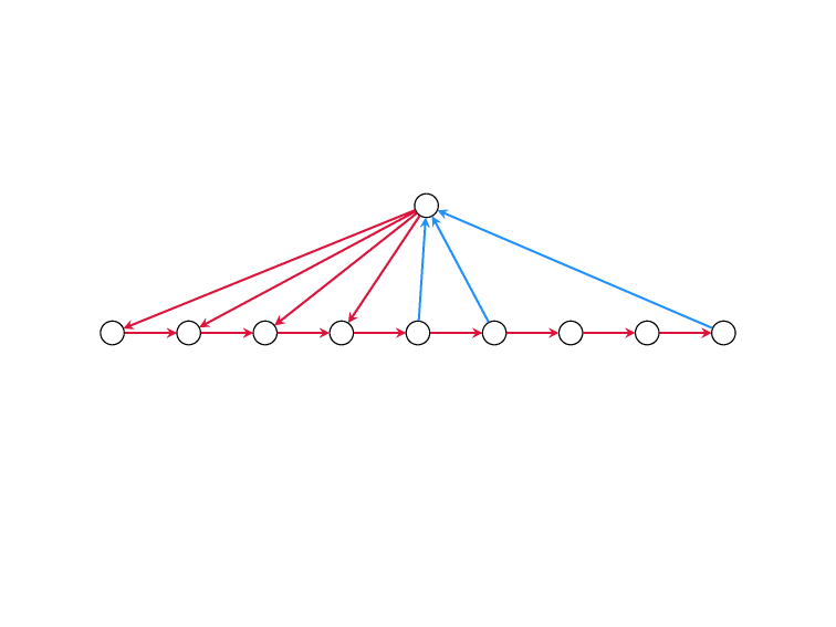
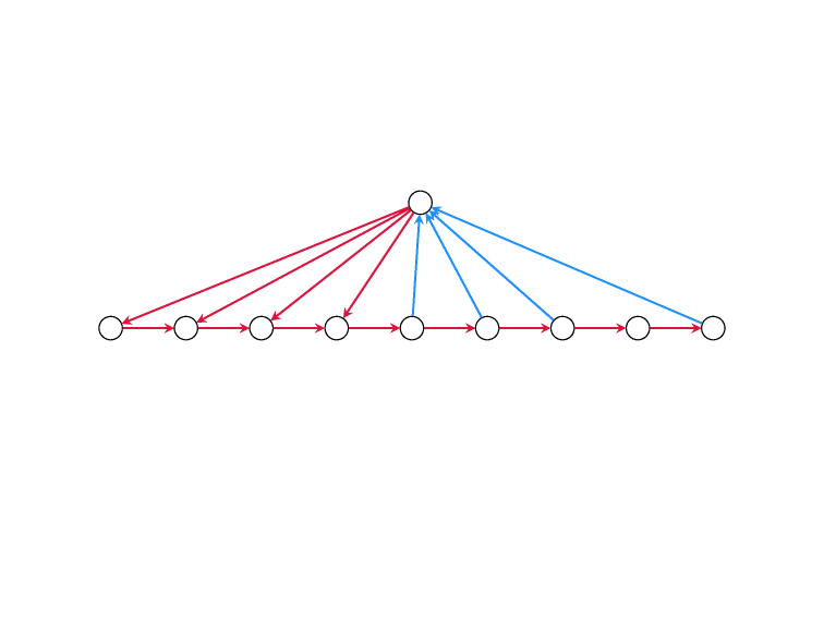
🍕
🍔
1
4


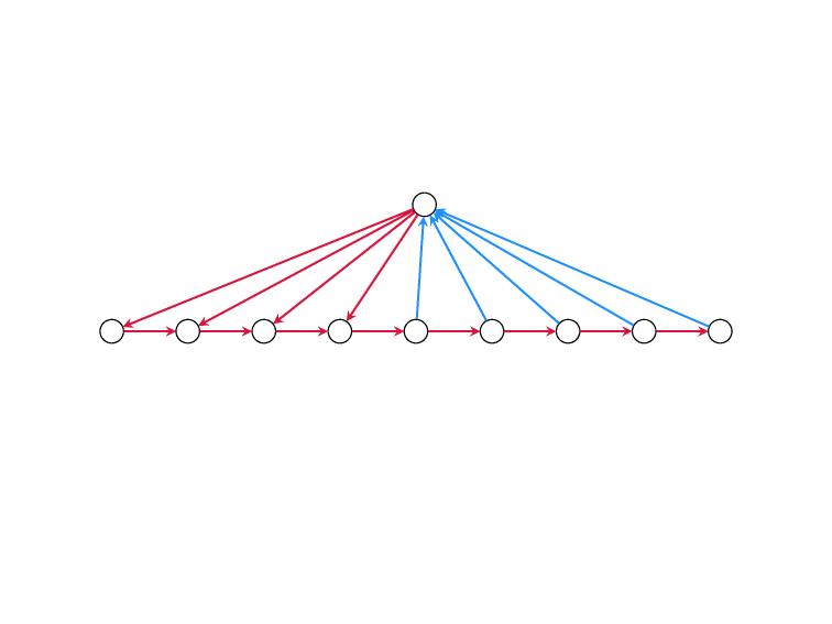

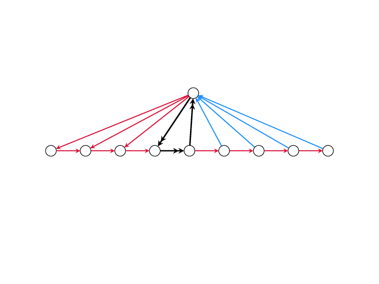

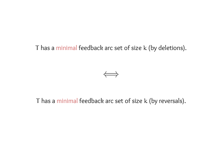
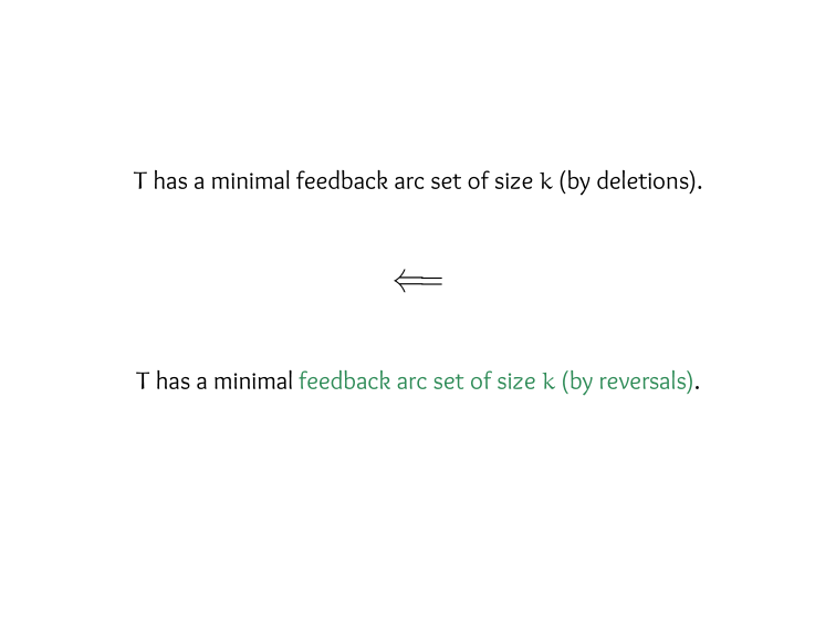
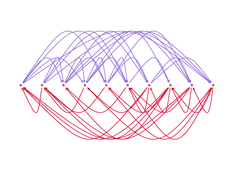

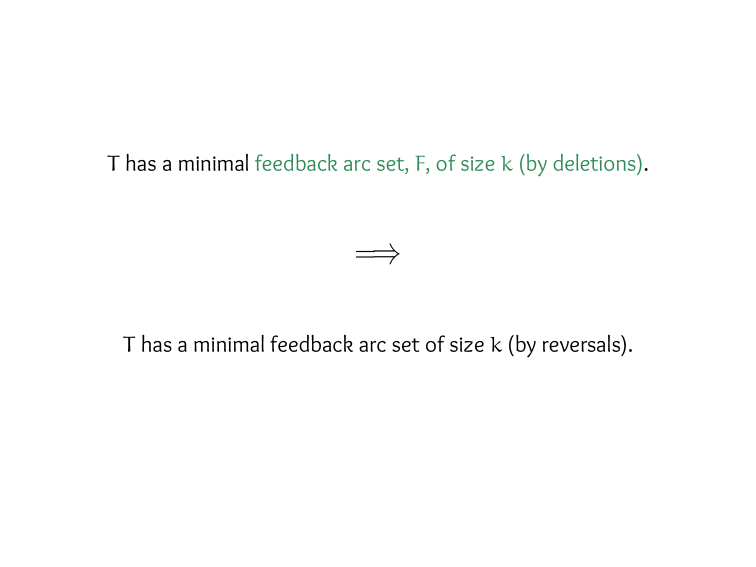
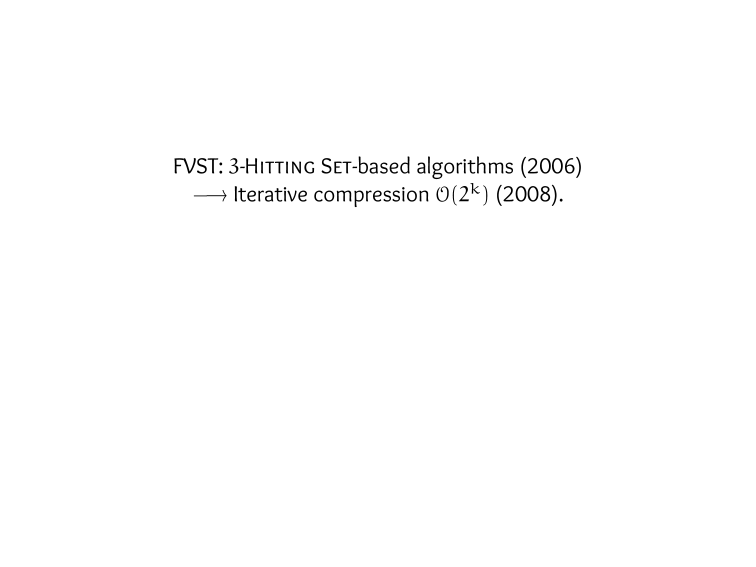
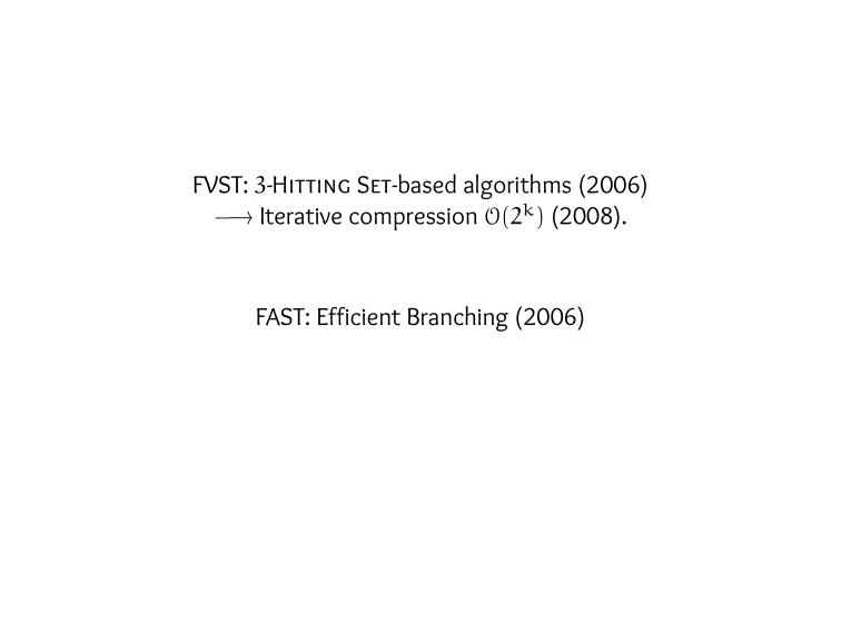
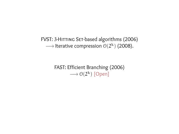
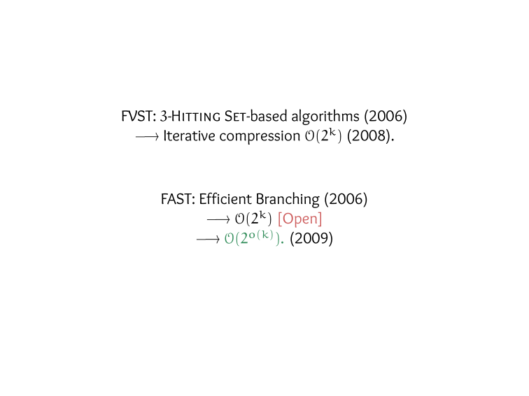


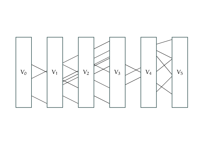
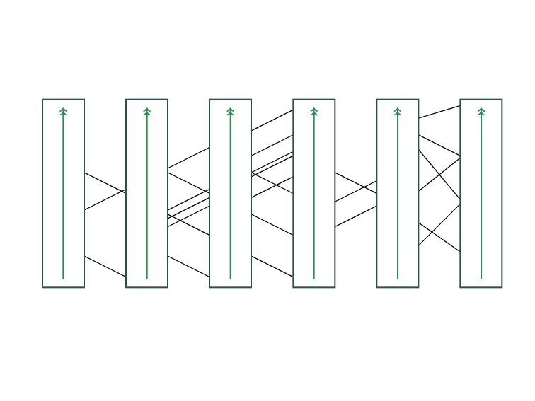

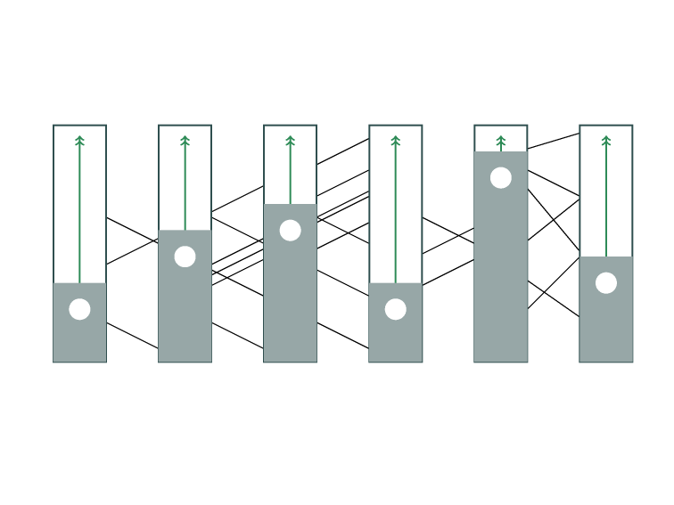
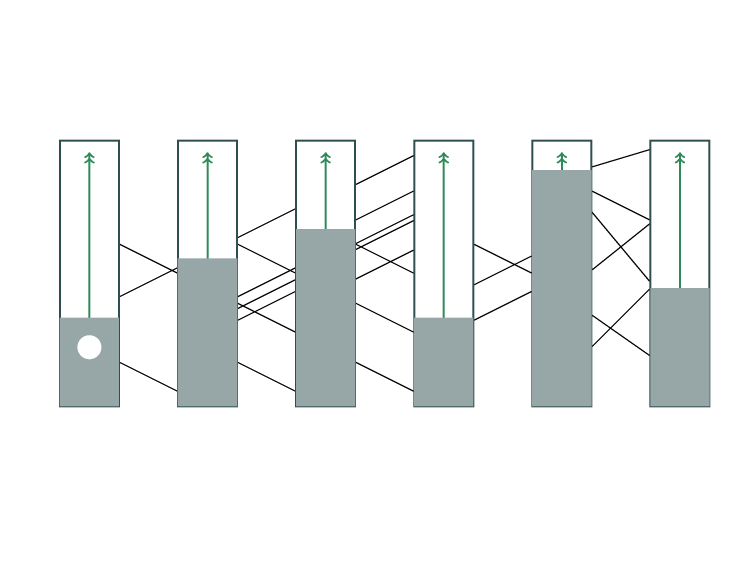




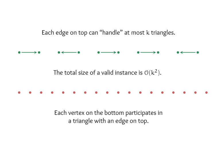
Decision Problems.
Does there exist at least one solution?
Search Problems.
Can you find me at least one solution?
Counting Problems.
How many solutions are there?
Enumeration Problems.
Enlist all the solutions.
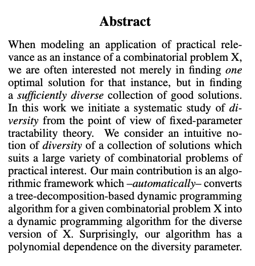
Diverse Problems.
Find me a useful bunch of solutions.


Completion Ordering Problem
(🍔 \(\succ\) 🍰), (🍩 \(\succ\) 🌮), etc.
Extend a given partial order to a total order,
given a cost function that associates a cost with every ordered pair of elements.
🍕 \(\succ\) 🍔 \(\succ\) 🍰 \(\succ\) 🍩 \(\succ\) 🌮
🍰 \(\succ\) 🍕 \(\succ\) 🌮 \(\succ\) 🍩 \(\succ\) 🍔
🍰 \(\succ\) 🍕 \(\succ\) 🍔 \(\succ\) 🍩 \(\succ\) 🌮
🌮 \(\succ\) 🍔 \(\succ\) 🍰 \(\succ\) 🍩 \(\succ\) 🍕
🌮 \(\succ\) 🍰 \(\succ\) 🍕 \(\succ\) 🍩 \(\succ\) 🍔
Partial Order: all unanimous pairs.
Cost of adding (🍔,🍕) = 4
Cost of adding (🍕,🍔) = 1
etc.
KRA → Completion Ordering
Parameter: pathwidth of the co-comparability graph of \(\rho\)
Main result: A DP-based algorithm for
Diverse Completion Ordering
that makes use of a \(\rho\)-consistent path decomposition.
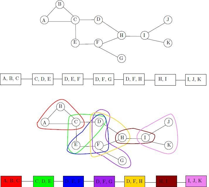
Path Decompositions as seen on Wikipedia
$$\mathcal{O}\left((\mathrm{w} ! \cdot \delta)^{\mathcal{O}(r)} \cdot s^{r^{2}} \cdot d \cdot n \cdot \log \left(n^{2} \cdot m\right)\right)$$
Running time for Diverse Completion Order
Also new: better running times for PCO
(not just the restriction to KRA)
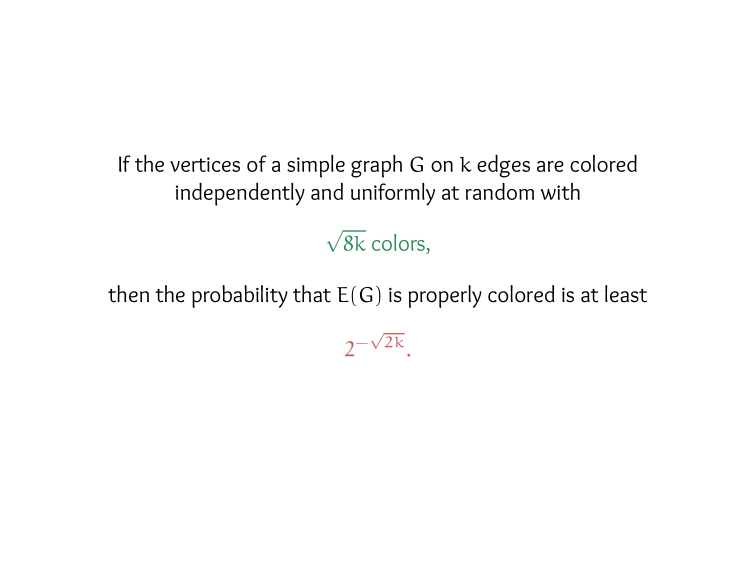
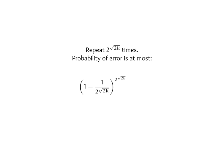
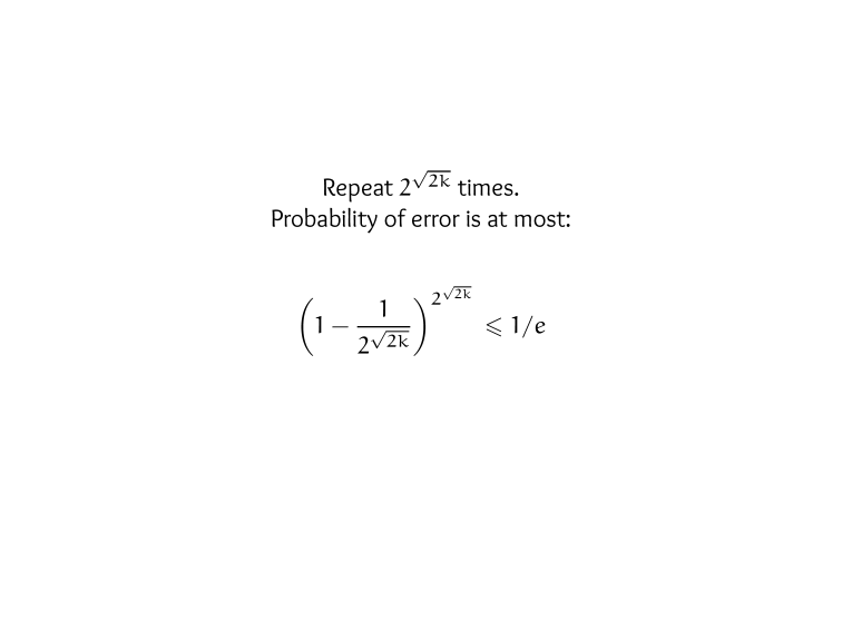
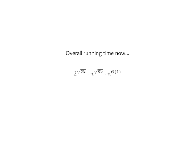
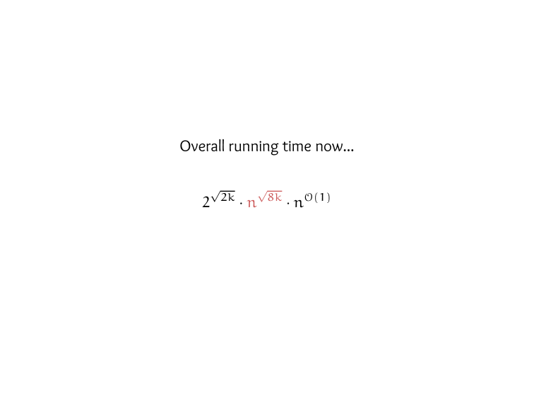
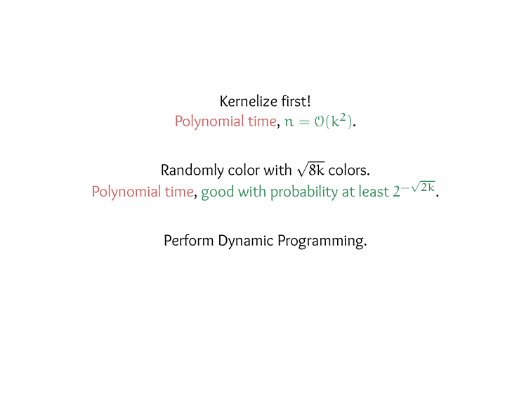
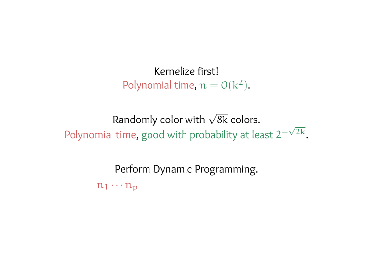
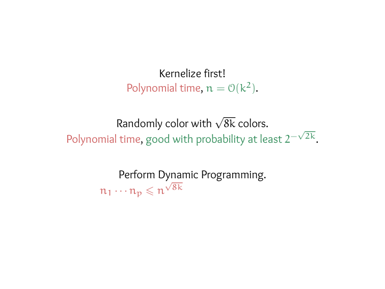
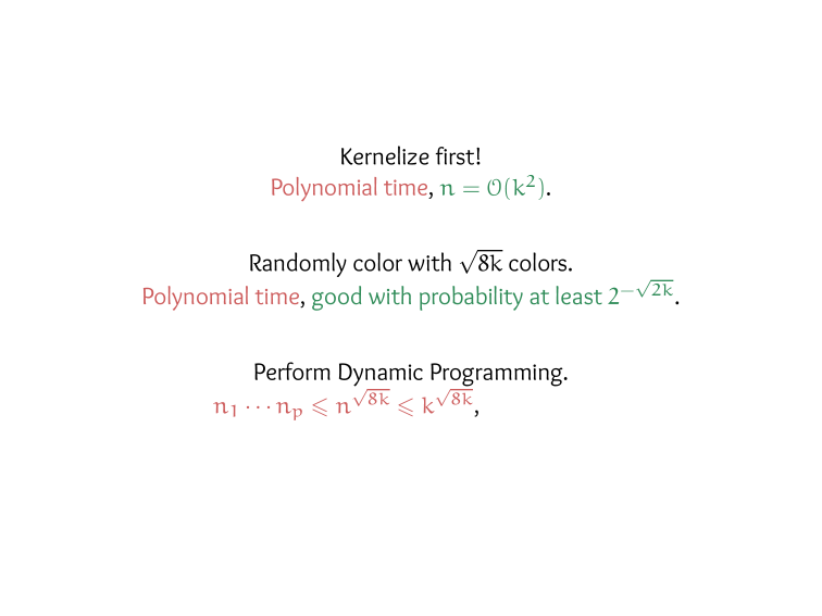
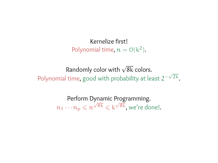
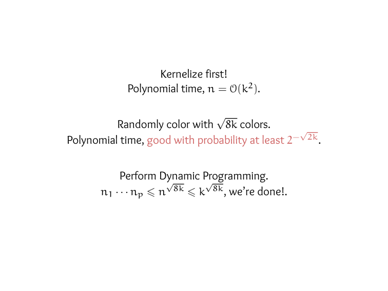
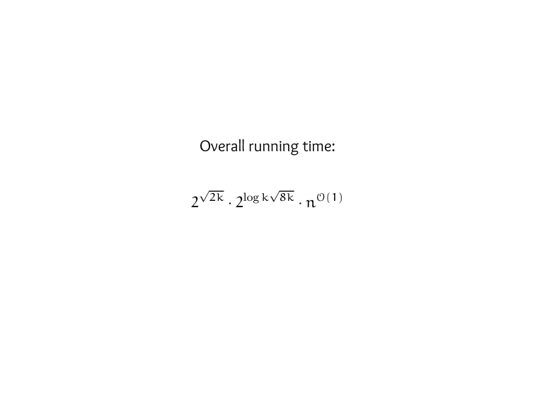
Given a partial order \(\rho \subseteq C \times C\) and a cost function \(\mathfrak{c}: C \times C \rightarrow \mathbb{N}\), one can solve a PCO instance \((\rho, \mathfrak{c}, k)\) in time \(|C| \cdot 2^{\mathcal{O}(\sqrt{k})}+\mathcal{O}\left(|C|^{2} \cdot \log (k)\right)\).
Takeaways
- KRA is a fundamental and fun rank aggregation problem that has connections with weighted FAST and PCO.
- Very well-studied from the approximation lens as well as from a parameterized perspective.
- Developments on diverse variants are recent and relevant; the space for exploring structural parameters is wide open.
Questions?
Thanks!
Parameterized KRA
By Neeldhara Misra
Parameterized KRA
- 703


