Random circuit sampling using fermionic linear optics


Michał Oszmaniec, ND, Mauro E. Morales, Zoltán Zimborás

The 5th Bangkok Workshop on Discrete Geometry, Dynamics and Statistics
24 Jan 2023



Matchgates!
Given an initial state \(|\psi\rangle\) and a family of unitary time evolutions \(\{U_{\alpha}\}_{\alpha}\),
are the \(U_{\alpha}|\psi\rangle\)'s hard to simulate on a classical computer?
-
Fundamental limit of classical computation
-
Direct applications are few and far between
- Certified random number generator (Aaronson)
- Company/Lab PR

pc: Reuters
- Introduction - What is a simulation?
- Proof strategy for classical intractability
- The fermionic case
Outline
String of \(n\) bits

Classical vs Quantum circuit
Output distribution over \(2^n\) bitstrings \(p({\bf x}) = p_{\bf x}\)

String of \(n\) qubits
Output distribution over \(2^n\) bitstrings \(p({\bf x}) = p_{\bf x}\)

Classical vs Quantum circuit

Output distribution over \(2^n\) bitstrings \(p({\bf x}) = p_{\bf x}\)
The result of the coin flips are just hidden bitstrings that can be included as extra inputs


Classical vs Quantum circuit

- Every Boolean circuit can be composed out of elementary gates in a universal gate set
- Most functions need an exponential-size circuit (Shannon)
- Every quantum circuit can be composed out of elementary gates in a universal gate set
- Most unitaries need an exponential-size circuit
Strong vs Weak Simulation


Strong simulation
Weak simulation
Can compute \(p_{\bf x}\)
Can sample from \(p\)
In practice, there need to be some notions of errors
In this talk, I will use these definitions of strong and weak simulation unless stated otherwise
Relative error
Additive error
Given an initial state \(|\psi\rangle\) and a family of unitary time evolutions \(\{U_{\alpha}\}_{\alpha}\), are the \(U_{\alpha}|\psi\rangle\)'s hard to simulate on a classical computer?
Given an initial state \(|\psi\rangle\) and a family of polynomial-depth quantum circuits \(\{U_{\alpha}\}_{\alpha}\), can there be a classical machine that approximately samples from \(p_{\bf x} = |\langle{\bf x}|U_{\alpha}|\psi\rangle|^2\) in poly\((n,\epsilon^{-1})\) time?
- Introduction - What is a simulation?
- Proof strategy for classical intractability
- The fermionic case
Outline
Proof of Classical Intractability
Given \(|\psi\rangle, \{U_{\alpha}\}_{\alpha}\)
If the RHS task is #P-hard, then \(\mathcal{C}^{\mathrm{NP}}\) would be able to solve a #P-hard problem, which we believe to be impossible
Classical sampler \(\mathcal{C}\)
Anti-concentration of \(p_{\bf x}(U_{\alpha})\)
Ability to approximately compute \(p_{\bf 0} = |\langle {\bf 0}|U_{\alpha}|\psi\rangle|^2\) for most \(U_{\alpha}\)
Anti-concentration
To turn relative error to additive error, we need most probabilities to be large
\(l^2\)-distance to the uniform distribution:
\(\Vert p-p_{\mathrm{unif}}\Vert^2 = Z - \displaystyle{\frac{1}{2^n}} = Z-Z_{\mathrm{unif}}\)
\(p_{\bf{x}}(U)\) anti-concentrates if
Implies \(\Pr\left(p_{{\bf x}} \ge \displaystyle{\frac{\beta}{2^n}}\right) \ge \alpha(1-\beta)^2 \) via the Paley-Zygmund inequality
Anti-concentration
Modified from Dalzell et al., PRX Quantum 2022
Average-Case Hardness
- Average-case hardness for Boson Sampling originates from the argument for average-case hardness to compute the permanent via polynomial interpolation (Lipton 1991).
- Bouland et al., Nat Phys (2018) and Movassagh 2019 import the argument to Random Circuit Sampling
Worst-case hardness of approximately computing \(p_{\bf 0}(U_{\alpha})\)
Worst-to-average-case reduction
Hardness of approximately computing \(p_{\bf 0}(U_{\alpha})\) for most \(U_{\alpha}\)
Easy to argue based on existing results in quantum computing
- Introduction - What is a simulation?
- Proof strategy for classical intractability
- The fermionic case
Outline

Rio Grande, 2017
Fermionic Linear Optics (FLO)
Reminder
Identify computational basis states with occupation number states

Jordan-Wigner
CAR
\(f_j^{\dagger}\) creates a fermion at site \(j\)
Pauli exclusion
Fermionic Linear Optics (FLO)
cf. Dirac's gamma matrices
Majoranas

Non-example
\(Z\!\otimes\! Z\) interaction is not FLO
FLO Hamiltonians are quadratic
Antisymmetric
Fermionic Linear Optics (FLO)
Even parity
Odd parity
FLO gates AKA Matchgates
(Valiant, SIAM J Comput 2002)
Non-example
Classical Intractability?
Classical sampler \(\mathcal{C}\)
Anti-concentration?
Ability to approximately compute \(p_{\bf 0} = |\langle {\bf 0}|V_{\mathrm{FLO}}|{\bf 0}\rangle|^2\) for most \(V_{\mathrm{FLO}}\)

This is easy!
Fermionic Linear Optics (FLO)
Generators of rotations SO(\(2n\))
(Defining representation)
Antisymmetric

Manipulating \(2n\times 2n\) matrices instead of \(2^n\times 2^n\) matrices!
- Only need to specify the correlation matrix (2nd moments)
- All higher moments can be extracted from \(\Sigma\) via Wick's theorem
\(\rho = (|0\rangle\langle 0|)^{\otimes n}\) is a fermionic Gaussian state
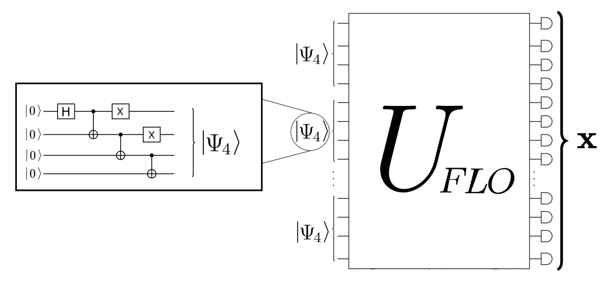
Fermion Sampling
- FLO with computational-basis input state admits strong simulation (compute \(p_{\bf x}\) up to logarithmic number of decimals)
- Not the case with non-Gaussian (magic) input state; strong simulation is #P-hard (cf. Ivanov, PRA 2017)
- Our work shows that weak simulation is also hard
Sum of projectors onto irreps by Schur's lemma under nice conditions
- SO(\(2n\)) for FLO
- U(\(n\)) for passive (number-preserving) FLO
Anti-concentration
For example,
Then use combinatorics to bound the RHS
Worst-to-average-case reduction
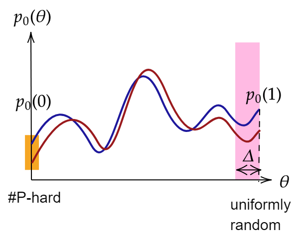
- There exists a "worst-case circuit" \(V_0\) for which \(p_{\bf 0} = |\langle \mathbf{0}|V_0|\Psi\rangle|^2\) is #P-hard to approximate
- Deform to average-case (Haar random) circuits where \(p_{\bf 0} (\theta)= |\langle \mathbf{0}|V(\theta)|\Psi\rangle|^2\) is a polynomial of low-degree \(q\)
- Sample \(\gtrsim q\) points (some can be errorneous\(\iff\)robustness) and recover \(p_{\bf 0}(\theta)\) via Berlekamp–Welch
- Plug in \(\theta = 0\) to solve a #P-hard problem!
Unitary Paths
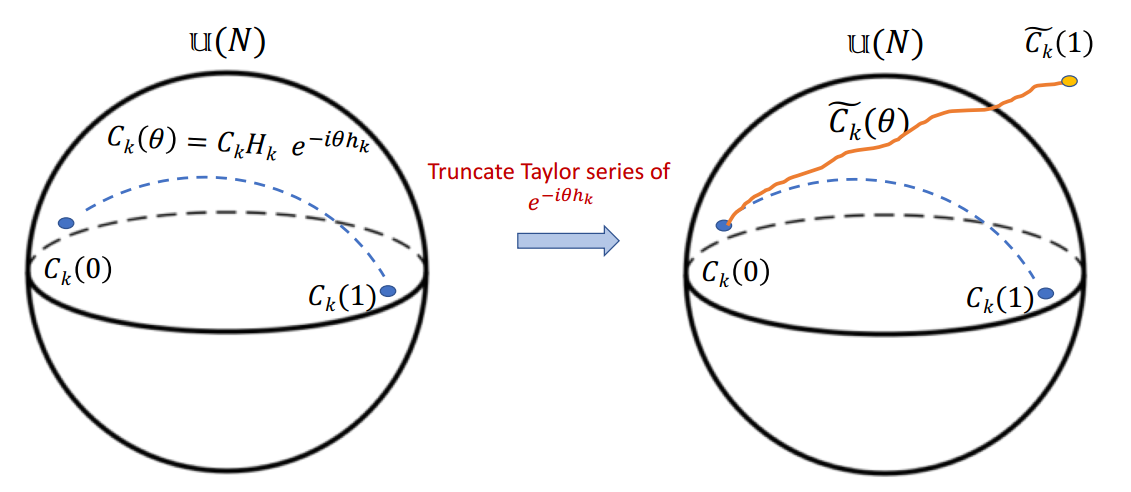
First idea: truncated exponential path
Movassage 2019
Truncation gives rise to a non-unitary operator
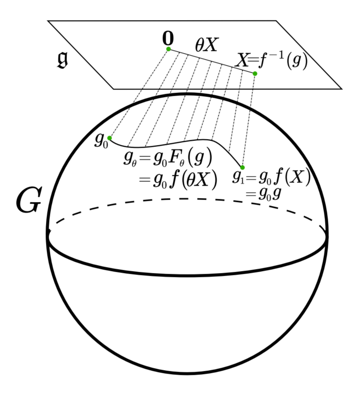
Better idea: Cayley path
Unitary
Hermitian
Hardness Guarantees
| Quantum advantage scheme | Robustness of avg-case hardness (additive error) |
Anti-concentration |
|---|---|---|
| Boson Sampling | ||
| Random circuit sampling (Google layout) | ||
| Fermion Sampling |


Bouland et al., FOCS 2021
Other Results
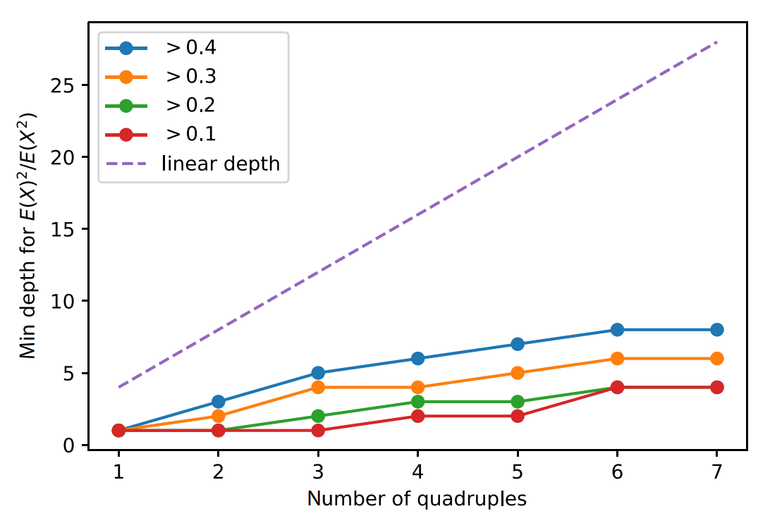
- Numerics suggest that random FLO circuits anti-concentrate in sub-linear depth
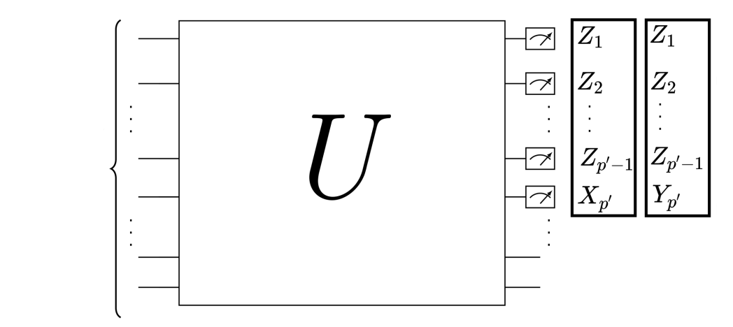
- Assuming that the circuit is FLO, circuit tomography can be performed efficiently utilizing single-mode input states and product measurements
Summary

- Simulating \(U|\psi\rangle\) = Sampling from \(|\langle {\bf x}|U|\psi\rangle|^2\)
- The standard argument for hardness of sampling requires statistical data of the ensemble \(\{U_{\alpha}\}_{\alpha}\)
- When \(\{U_{\alpha}\}_{\alpha}\) has the structure of a low-dimensional Lie group, there are available techniques for computing these data
- Low-dimensionality might lead to a fast classical algorithm; but this might be circumvented by a good choice of the initial state (here a non-Gaussian state)
Thank You!

↑ for the slides
Fermion Sampling (DGDS2023)
By Ninnat Dangniam
Fermion Sampling (DGDS2023)
The 5th Bangkok Workshop on Discrete Geometry, Dynamics and Statistics (23-27 Jan 2023)
- 508


