Machine Learning
機器學習
講師 000

技能樹
-
Full Stack
-
Discord Bot
-
Machine Learning
-
Unity
-
Competitive Programming
-
Web Crawler
-
Server Deployment
-
Minecraft Datapack -
Scratch
-
Intro
-
Linear Algebra
-
Partial Derivative
-
Activation Function
-
Neural Network
-
Loss Function
-
Optimization
目錄
-
Backpropagation
-
Programing
-
Training
-
Problems
Intro
介紹
什麼是機器學習?

什麼是機器學習?
機器會學習什麼?
什麼是學習?
聽起來很厲害?
它是怎麼學習的?
上一堂課的講師為什麼那麼甲?
深度學習又是啥?
它是新東西嗎?
機器學習
Machine Learning
機器學習
Machine Learning
利用統計數據去推論出結果
這也是被視為「學習」的動作
機器學習
Machine Learning
而實現機器學習的演算法有非常多種
其中我們常聽到的模型都是基於神經網路
而這便是深度學習的範疇
深度學習
Deep Learning
標準神經網路
深度學習
Deep Learning
標準神經網路
深度學習
Deep Learning
遞迴神經網路
標準神經網路
深度學習
Deep Learning
遞迴神經網路
卷積神經網路
標準神經網路
深度學習
Deep Learning
遞迴神經網路
卷積神經網路


大語言模型
注意力機制
本次課程將會由原理開始帶大家理解並實作
一切的根源--標準神經網路
深度學習
Deep Learning
Linear Algebra
線性代數
純量
X = 10
沒有方向性的元素
剛剛矩陣內的每一個元素都是一個純量
Scalar
向量
\vec X_{n} =
\left[
\begin{matrix}
x_{0} \\
x_{1} \\
\vdots \\
x_{n} \\
\end{matrix}
\right]
只有一維的矩陣
同時表示著一個空間中的向量
Vector
張量
\vec X_{mn} =
\left[
\begin{matrix}
x_{00} & x_{10} & \cdots & x_{m0}\\
x_{01} & x_{11} & \cdots & x_{m1}\\
\vdots & \vdots & \cdots & \vdots\\
x_{0n} & x_{1n} & \cdots & x_{mn}\\
\end{matrix}
\right]
數個向量構成的矩陣
Tensor
內積
\vec X =
\left[
\begin{matrix}
x_{0} \\
x_{1} \\
\vdots \\
x_{n} \\
\end{matrix}
\right]
兩個向量進行內積時
會如矩陣乘法一般將兩向量每個元素相乘
只不過最後得到的輸出不是矩陣
而是元素相乘值的總和(純量)
Dot Product
\vec Y =
\left[
\begin{matrix}
y_{0} \\
y_{1} \\
\vdots \\
y_{n} \\
\end{matrix}
\right]
\vec X \cdot \vec Y = \sum_{i=0}^{n} x_i y_i
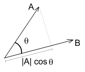
內積
\vec X \cdot \vec Y = |{\vec X}| |{\vec Y}| \cos \theta
在幾何意義上它代表的是 X 向量在 Y 向量上的投影長與 Y 向量長度的積
Dot Product
矩陣
x =
\left[
\begin{matrix}
1 & 2 \\
3 & 4 \\
\end{matrix}
\right]
Matrix
矩陣
x =
\left[
\begin{matrix}
1 & 2 \\
3 & 4 \\
\end{matrix}
\right]
Matrix
就是一個包含許多數字的東東
其中每一個數字都被稱作是矩陣的元素
矩陣計算
\left[
\begin{matrix}
1 & 2 \\
3 & 4 \\
\end{matrix}
\right]
+ 5 =
\left[
\begin{matrix}
6 & 7 \\
8 & 9 \\
\end{matrix}
\right]
矩陣計算
\left[
\begin{matrix}
1 & 2 \\
3 & 4 \\
\end{matrix}
\right]
+ 5 =
\left[
\begin{matrix}
6 & 7 \\
8 & 9 \\
\end{matrix}
\right]
很簡單吧
矩陣計算
\left[
\begin{matrix}
1 & 2 \\
3 & 4 \\
\end{matrix}
\right]
* 5 =
\left[
\begin{matrix}
5 & 10 \\
15 & 20 \\
\end{matrix}
\right]
矩陣計算
\left[
\begin{matrix}
1 & 2 \\
3 & 4 \\
\end{matrix}
\right]
* 5 =
\left[
\begin{matrix}
5 & 10 \\
15 & 20 \\
\end{matrix}
\right]
如果運算的對象是矩陣呢?
矩陣計算
\left[
\begin{matrix}
1 & 2 \\
3 & 4 \\
\end{matrix}
\right]
+
\left[
\begin{matrix}
5 & 6\\
7 & 8 \\
\end{matrix}
\right]
=
\left[
\begin{matrix}
1+5 & 2+6 \\
3+7 & 4+8 \\
\end{matrix}
\right]
兩個矩陣需要一樣形狀
A_{mn} \\
B_{mn}
矩陣計算
如果是乘法呢?
轉置矩陣
A =
\left[
\begin{matrix}
1 & 2 & 3\\
4 & 5 & 6\\
\end{matrix}
\right]
A^{T} =
\left[
\begin{matrix}
1 & 4 \\
2 & 5 \\
3 & 6 \\
\end{matrix}
\right]
轉置矩陣
A =
\left[
\begin{matrix}
1 & 2 & 3\\
4 & 5 & 6\\
\end{matrix}
\right]
A^{T} =
\left[
\begin{matrix}
1 & 4 \\
2 & 5 \\
3 & 6 \\
\end{matrix}
\right]
轉置矩陣
A =
\left[
\begin{matrix}
1 & 2 & 3\\
4 & 5 & 6\\
\end{matrix}
\right]
A^{T} =
\left[
\begin{matrix}
1 & 4 \\
2 & 5 \\
3 & 6 \\
\end{matrix}
\right]
轉置矩陣
A =
\left[
\begin{matrix}
1 & 2 & 3\\
4 & 5 & 6\\
\end{matrix}
\right]
A^{T} =
\left[
\begin{matrix}
1 & 4 \\
2 & 5 \\
3 & 6 \\
\end{matrix}
\right]
轉置矩陣
B =
\left[
\begin{matrix}
1 & 2 \\
3 & 4 \\
\end{matrix}
\right]
B^{T} =
\left[
\begin{matrix}
1 & 3 \\
2 & 4 \\
\end{matrix}
\right]
轉置矩陣
B =
\left[
\begin{matrix}
1 & 2 \\
3 & 4 \\
\end{matrix}
\right]
B^{T} =
\left[
\begin{matrix}
1 & 3 \\
2 & 4 \\
\end{matrix}
\right]
轉置矩陣
B =
\left[
\begin{matrix}
1 & 2 \\
3 & 4 \\
\end{matrix}
\right]
B^{T} =
\left[
\begin{matrix}
1 & 3 \\
2 & 4 \\
\end{matrix}
\right]
矩陣乘法
\left[
\begin{matrix}
1 & 2 & 3\\
4 & 5 & 6\\
\end{matrix}
\right]
\cdot
\left[
\begin{matrix}
5 & 6 \\
7 & 8 \\
9 & 10\\
\end{matrix}
\right]
=\left[
\begin{matrix}
(1 \times 5 + 2 \times 7 + 3 \times 9)&
(1 \times 6 + 2 \times 8 + 3 \times 10)\\
(4 \times 5 + 5 \times 7 + 6 \times 9)&
(4 \times 6 + 5 \times 8 + 6 \times 10)\\
\end{matrix}
\right]
順帶一提這東西沒有交換律
Partial Derivative
偏微分
斜率
Slope
斜率
Slope
m = \frac{\Delta y}{\Delta x}
斜率
Slope
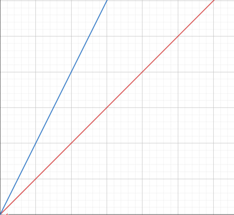
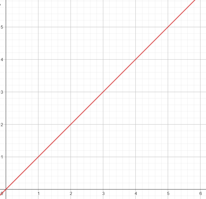
m=2
m=1
斜率
Slope
m = Undefined
m = 0
微分
Differential
如果我要求函數中無限趨近於一個點上的斜率怎麼做
微分
Differential
如果我要求函數中無限趨近於一個點上的斜率怎麼做
設定
\lim_{\Delta X \to 0} X + \Delta X = X'
微分
Differential
\lim_{\Delta X \to 0} X + \Delta X = X'
Y
X
微分
Differential
\lim_{\Delta X \to 0} X + \Delta X = X'
Y
X
x
x'
微分
Differential
\lim_{\Delta X \to 0} X + \Delta X = X'
Y
X
x
x'
Δx
微分
Differential
\lim_{\Delta X \to 0} X + \Delta X = X'
Y
X
x
x'
Δx
y
y
Δy
y'
微分
\lim_{\Delta X \to 0} \frac{Y + \Delta Y - Y}{X + \Delta X - X}
Y
X
x
x'
Δx
y
y'
y
Δy
Differential
微分
\lim_{h \to 0} \frac{f(x+h) - f(x)}{X + h - X}
Differential
微分
\lim_{h \to 0} \frac{f(x+h) - f(x)}{h}
Differential
微分
f(x)^{'} = \lim_{h \to 0} \frac{f(x+h) - f(x)}{h}
Differential
微分
\frac{\mathrm{d} y}{\mathrm{d} x} = f(x)^{'} = \lim_{h \to 0} \frac{f(x+h) - f(x)}{h}
Differential
微分
Differential
f(x) = 114514 \\
f(x) = x \\
f(x) = ax^b + c
微分
Differential
f(x) = 114514 \\
微分
Differential
f(x) = 114514 \\
\lim_{h \to 0} \frac{f(x+h) - f(x)}{h}
微分
Differential
f(x) = 114514 \\
\lim_{h \to 0} \frac{114514 - 114514}{h}
微分
Differential
f(x) = 114514 \\
\lim_{h \to 0} \frac{114514 - 114514}{h} = 0
微分
Differential
f(x) = 114514 \\
Y
X
m = 0
微分
Differential
f(x) = x \\
微分
Differential
f(x) = x \\
\lim_{h \to 0} \frac{f(x+h) - f(x)}{h}
微分
Differential
f(x) = x \\
\lim_{h \to 0} \frac{x+h - x}{h}
微分
Differential
f(x) = x \\
\lim_{h \to 0} \frac{h}{h} = 1
微分
Differential
f(x) = ax^b + c
微分
Differential
f(x)^{'} = \frac{\mathrm{d} (ax^b + c)}{\mathrm{d} x} \\
微分
Differential
f(x)^{'} = \frac{\mathrm{d} (ax^b + c)}{\mathrm{d} x} \\
= \frac{\mathrm{d} (ax^b)}{\mathrm{d} x} + \frac{\mathrm{d} c}{\mathrm{d} x}
= a\frac{\mathrm{d} (x^b)}{\mathrm{d} x} + \frac{\mathrm{d} c}{\mathrm{d} x}
微分
Differential
f(x)^{'} = \frac{\mathrm{d} (ax^b + c)}{\mathrm{d} x} \\
= \frac{\mathrm{d} (ax^b)}{\mathrm{d} x} + \frac{\mathrm{d} c}{\mathrm{d} x}
= a\frac{\mathrm{d} (x^b)}{\mathrm{d} x} + \frac{\mathrm{d} c}{\mathrm{d} x}
= 0
微分
Differential
g(x) = x^b
\lim_{h \to 0} \frac{g(x+h) - g(x)}{h}
微分
Differential
g(x) = x^b
\lim_{h \to 0} \frac{(x+h)^b - x^b}{h}
微分
Differential
g(x) = x^n
\lim_{h \to 0} \frac{(x+h)^n - x^n}{h}
微分
Differential
g(x) = x^n
\lim_{h \to 0} \frac{(x+h)^n - x^n}{h}
= \lim_{h \to 0} \frac{
\sum^{n}_{k=0} {
\left(
\begin{matrix}
n \\ k
\end{matrix}
\right)
x^{n-k} h^k
}- x^n}{h}
微分
Differential
= \lim_{h \to 0} \frac{
\sum^{n}_{k=0} {
\left(
\begin{matrix}
n \\ k
\end{matrix}
\right)
x^{n-k} h^k
}- x^n}{h}
= \lim_{h \to 0} \frac{
(1)x^{n-0} h^0
+
(n)x^{n-1} h^1
+
...
- x^n}{h}
微分
Differential
= \lim_{h \to 0} \frac{
\sum^{n}_{k=0} {
\left(
\begin{matrix}
n \\ k
\end{matrix}
\right)
x^{n-k} h^k
}- x^n}{h}
= \lim_{h \to 0} \frac{
(1)x^{n-0} h^0
+
(n)x^{n-1} h^1
+
...
- x^n}{h}
微分
Differential
= \lim_{h \to 0} \frac{
nx^{n-1} h^1
+
...
}{h}
微分
Differential
= \lim_{h \to 0} \frac{
nx^{n-1} h^1
+
...
}{h}
= nx^{n-1}
微分
Differential
= \lim_{h \to 0} \frac{
nx^{n-1} h^1
+
...
}{h}
= nx^{n-1}
後面幾項都因為有h作為係數而歸零了
微分
Differential
f(x) = ax^b + c
f(x)^{'} = abx^{b-1}
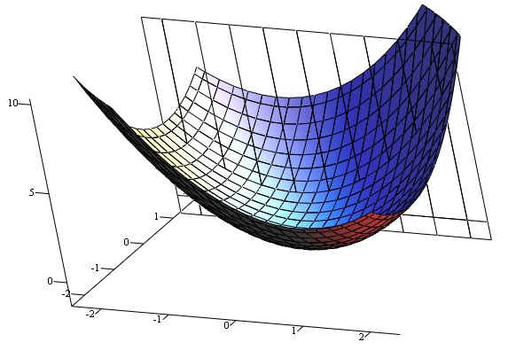
梯度
Gradient
而若是這樣一個非二維的空間中
我們想要知道圖形上任意點
在特定軸上的斜率
同時也代表的該參數與圖形的關係
偏微分
Partial Differential
在一個多變數的方程式中求特定變數的微分
偏微分
Partial Differential
在一個多變數的方程式中求特定變數的微分
f(x) = x^2 + xy + y^2
偏微分
Partial Differential
在一個多變數的方程式中求特定變數的微分
\frac{\partial f(x)}{\partial x}
f(x) = x^2 + xy + y^2
偏微分
Partial Differential
在一個多變數的方程式中求特定變數的微分
f(x) = x^2 + xy + y^2
\frac{\partial f(x)}{\partial x} =
\frac{\partial (
x^2 + xy + y^2
)}{\partial x}
偏微分
Partial Differential
f(x) = x^2 + xy + y^2
=
\frac{\partial (
x^2 + x^1y + x^0y^2
)}{\partial x}
\frac{\partial f(x)}{\partial x} =
\frac{\partial (
x^2 + xy + y^2
)}{\partial x}
偏微分
Partial Differential
f(x) = x^2 + xy + y^2
=
\frac{\partial (
x^2 + x^1y + x^0y^2
)}{\partial x}
\frac{\partial f(x)}{\partial x} =
\frac{\partial (
x^2 + xy + y^2
)}{\partial x}
= 2x + 1y + 0y^2
偏微分
Partial Differential
f(x) = x^2 + xy + y^2
=
\frac{\partial (
x^2 + x^1y + x^0y^2
)}{\partial x}
\frac{\partial f(x)}{\partial x} =
\frac{\partial (
x^2 + xy + y^2
)}{\partial x}
= 2x + 1y + 0y^2 = 2x+y
偏微分
Partial Differential
f(x) = x^2 + xy + y^2
\frac{\partial f(x)}{\partial x} = 2x+y
Activation Function
激勵函數 / 啟動函數
神經元
\vec X
Y
Neuron
\sigma(
(\sum_{i=1}^{n}
x_i \times w_i) +b)
\vec X
Y
\sigma(
(\sum_{i=1}^{n}
x_i \times w_i) +b)
\vec X
Y
讓他好看一點
=
\sigma( \left[
\begin{matrix}
x_{0} \\
x_{1} \\
\vdots \\
x_{n} \\
\end{matrix}
\right]
\cdot
\left[
\begin{matrix}
w_{0} &
w_{1}
\cdots
w_{n}
\end{matrix}
\right]
+
b)
\vec X
Y
\sigma(\vec X \cdot \vec W + b) = Y
\vec X
Y
\sigma(\vec X \cdot \vec W + b) = Y
\vec X
Y
這就是每個Neuron在進行的事情
\sigma(\vec X \cdot \vec W + b) = Y
\vec X
Y
這就是每個Neuron在進行的事情
把輸入( X )乘上一個Weight並且加上Bias
\sigma (\vec X \cdot \vec W + b) = Y
\vec X
Y
這就是每個Neuron在進行的事情
把輸入( X )乘上一個Weight並且加上Bias
最後在套上本章的主角 Activation Function
class Neuron:
    def __init__(self, w: np.ndarray, b: int) -> None:
        self.w = w
        self.b = b

    def forward(self, x) -> int:
        return relu(np.dot(x, self.w.T) + self.b)
#$%#*@)$!#)$%(#)$%
Neuron Code
Activation Function
如果一直進行wx+b的操作會發現它始終是線性的,這樣一來這整個神經網路能夠擬合出來的函式會被限縮
而激勵函數能夠提供給這個神經網路的方程式非線性的來改善這個問題
Activation Function
如果一直進行wx+b的操作會發現它始終是線性的,這樣一來這整個神經網路能夠擬合出來的函式會被限縮
而激勵函數能夠提供給這個神經網路的方程式非線性的來改善這個問題
並且能夠對每個神經元輸出的值進行一定程度的控制
例如: 限縮範圍,限縮負數成長
Activation Function
-
Identity
-
Binary step
-
Sigmoid
-
tanh
-
ReLU
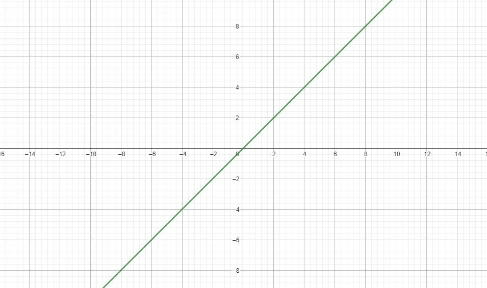
Identity
\sigma(x) = x
Identity
def Identity(x):
  	return x
#$%#*@)$!#)$%(#)$%
Identity Code
這有必要放嗎
※幾乎不會用到
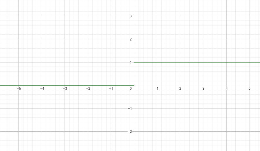
Binary step / Sign
\sigma(x) =
\begin{cases}
0 &
\text{if $x$ $\lt$ 0 }
\\
1 &
\text{if $x$ $\ge$ 0 } \\
\end{cases}
def sign(x):
    return 1 if x >= 0 else 0
#$%#*@)$!#)$%(#)$%
Sign Code
#matrix
def sign(x):
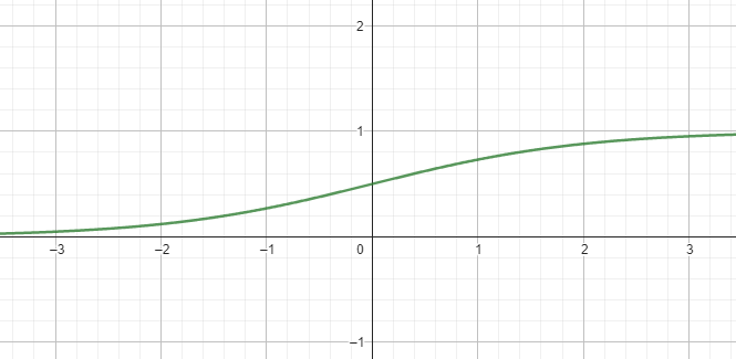
return 1 * (x >= 0)Sigmoid
\sigma(x) =
\frac
{1}
{1+e^{-x}}
def sigmoid(x):
    return 1 / (1 + np.exp(-x))
#$%#*@)$!#)$%(#)$%
Sigmoid Code
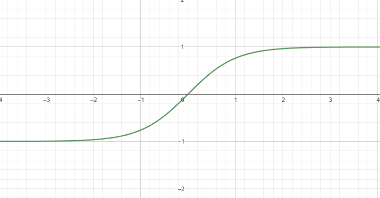
tanh
\sigma(x) =
tanh(x) =
\frac
{e^{x} - e^{-x}}
{e^{x} + e^{-x}}
def tanh(x):
    return np.tanh(x)
#$%#*@)$!#)$%(#)$%
tanh Code
貼心的numpy已經有現成的了
ReLU
\sigma(x) =
\begin{cases}
0 &
\text{if $x$ $\le$ 0 }
\\
x &
\text{if $x$ $\gt$ 0 } \\
\end{cases}
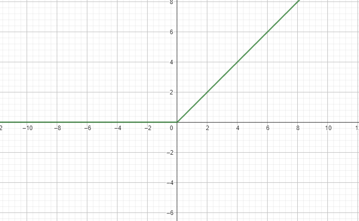
ReLU
\sigma(x) =
max(0, x)
def relu(x):
    return np.maximum(0, x)

def leaky_relu(x, n: float=1e-3):
    return x if max(0, x) else n*x
#$%#*@)$!#)$%(#)$%
ReLU Code
簡單提一下Leaky ReLU
它會將小於0的數字乘上一個很小的數字
讓負數也能保留數值之間的差距而不是直接歸0
Softmax
\sigma_{i} (\vec x) =
\frac
{e^{x_{i}}}
{\sum\limits_{j=0}^{J} e^{x_{j}}}
Softmax
\sigma_{i} (\vec x) =
\frac
{e^{x_{i}}}
{\sum\limits_{j=0}^{J} e^{x_{j}}}
它使用於Output layer
會將每項輸出層神經元的數值做e^x之後
計算在總和之間的比例
Softmax
簡單來說
每個輸出層神經元的數值總和會是1
可以用來做比例 / 機率分配等應用
\sigma_{i} (\vec x) =
\frac
{e^{x_{i}}}
{\sum\limits_{j=0}^{J} e^{x_{j}}}
Softmax
嗯我知道還是很難懂
\sigma_{i} (\vec x) =
\frac
{e^{x_{i}}}
{\sum\limits_{j=0}^{J} e^{x_{j}}}
Softmax
讓我們來直接看看範例
嗯我知道還是很難懂
\sigma_{i} (\vec x) =
\frac
{e^{x_{i}}}
{\sum\limits_{j=0}^{J} e^{x_{j}}}
Softmax
e^{\vec x} =
\left[
\begin{matrix}
1 \\
2 \\
3 \\
\end{matrix}
\right]
\frac
{1}
{1+2+3}
\text{、}
\frac
{2}
{1+2+3}
\text{、}
\frac
{3}
{1+2+3}
\sigma_{i} (\vec x) =
\frac
{e^{x_{i}}}
{\sum\limits_{j=0}^{J} e^{x_{j}}}
Softmax
\frac
{1}
{6}
\text{、}
\frac
{2}
{6}
\text{、}
\frac
{3}
{6}
\sigma_{i} (\vec x) =
\frac
{e^{x_{i}}}
{\sum\limits_{j=0}^{J} e^{x_{j}}}
e^{\vec x} =
\left[
\begin{matrix}
1 \\
2 \\
3 \\
\end{matrix}
\right]
Softmax
\frac
{1}
{6}
+
\frac
{2}
{6}
+
\frac
{3}
{6}
= 1
\sigma_{i} (\vec x) =
\frac
{e^{x_{i}}}
{\sum\limits_{j=0}^{J} e^{x_{j}}}
e^{\vec x} =
\left[
\begin{matrix}
1 \\
2 \\
3 \\
\end{matrix}
\right]
Softmax
\frac{1}{6}
\frac{3}{6}
\frac{2}{6}
=1
Softmax
那可以做什麼呢?
Softmax
那可以做什麼呢?


Softmax
那可以做什麼呢?
\frac{1}{6}
\frac{2}{6}
\frac{3}{6}
Softmax
那可以做什麼呢?

def softmax(x):
    return np.exp(x) / np.sum(np.exp(x))
#$%#*@)$!#)$%(#)$%
Softmax Code
def softmax(x):
    return np.exp(x - np.max(x) / np.sum(np.exp(x - np.max(x)))
Neural Network
神經網路
想想如果一堆Neuron合起來會變成什麼呢?
layer
\vec X
\vec Y
layer
\sigma(\vec X \cdot \vec W + \vec B) = \vec Y
\vec X
\vec Y
\vec X \cdot \vec W + \vec B
\sigma(\vec X \cdot \vec W + \vec B) = \vec Y
\vec X
\vec Y
=
\left[
\begin{matrix}
x_{00} & x_{10} & \cdots & x_{m0}\\
x_{01} & x_{11} & \cdots & x_{m1}\\
\vdots & \vdots & \cdots & \vdots\\
x_{0n} & x_{1n} & \cdots & x_{mn}\\
\end{matrix}
\right]
\cdot
\left[
\begin{matrix}
w_{0} \\
w_{1} \\
\vdots \\
w_{n} \\
\end{matrix}
\right]
+
\left[
\begin{matrix}
b_{0} \\
b_{1} \\
\vdots \\
b_{n} \\
\end{matrix}
\right]
\sigma(\vec X \cdot \vec W + \vec B) = \vec Y
\vec X
\vec Y
Neural Network
#&#%(@$#@)*%
Neural Network
#&#%(@$#@)*%
Neural Network
#&#%(@$#@)*%
#&#%(@$#@)*%
#&#%(@$#@)*%
Input Layer
#&#%(@$#@)*%
Input Layer
Hidden Layer
#&#%(@$#@)*%
Input Layer
Hidden Layer
Output Layer
#&#%(@$#@)*%
Input Layer
Hidden Layer
Output Layer
#&#%(@$#@)*%
\vec X
\vec Y
Input Layer
Hidden Layer
Output Layer
#&#%(@$#@)*%
\vec X
\vec Y
我們的目的就是幫要解決的問題
找出一個完美的函式
使同一類問題的輸入都能夠得到正確的輸出
#&#%(@$#@)*%
\vec X
\vec Y
但是我要怎麼知道
每個神經元的參數應該要是多少呢?
我們的目的就是幫要解決的問題
找出一個完美的函式
使同一類問題的輸入都能夠得到正確的輸出
Loss Function
損失函數
\vec X
\vec Y
\vec X
\vec Y
如何讓他們成為應該成為這個
目標函式的正確參數?
很多的權重與偏移
\vec X
\vec Y
先隨便帶入任意數字
\vec X
\vec Y
\vec X
\vec Y
\text{將} \vec X帶入
\vec X
\vec Y
\vec X
\vec Y
\text{得到} \vec Y_{output}
\text{用} \vec Y_{output} 與 \vec Y_{ans} 計算Loss
再根據Loss去調整 \vec W, \vec B
\text{用} \vec Y_{output} 與 \vec Y_{ans} 計算Loss
再根據Loss去調整 \vec W, \vec B
而Loss Function就是用來
計算Loss的函式
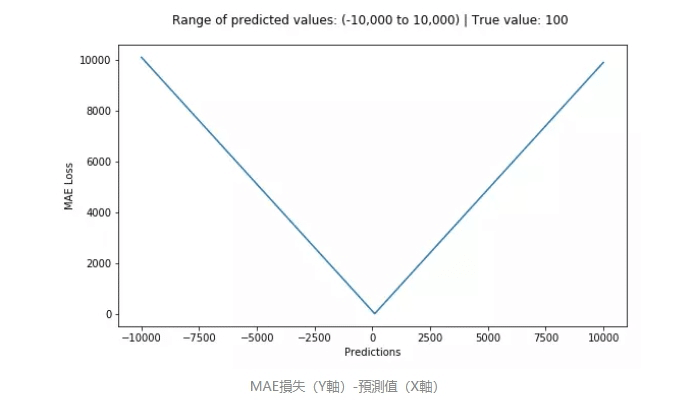
Mean Absolute Error
\text{MAE} =
\frac
{1}
{n}
\sum_{i=1}^{n}
|y_{i} - \hat y_{i} |
平均絕對值誤差
Mean Square Error
平均平方誤差 / 均方誤差
\text{MSE} =
\frac
{1}
{n}
\sum_{i=1}^{n}
(y_{i} - \hat y_{i} )^2
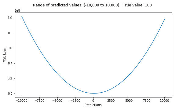
\text{MAE}
\text{MSE}
交叉熵
Cross Entropy
-\sum_{i}
\hat y_{i} \log_{2} y_{i}
交叉熵
Cross Entropy
為正確的數據
為輸出的數據
\hat y
y
-\sum_{i}
\hat y_{i} \log_{2} y_{i}
Cross Entropy
交叉熵
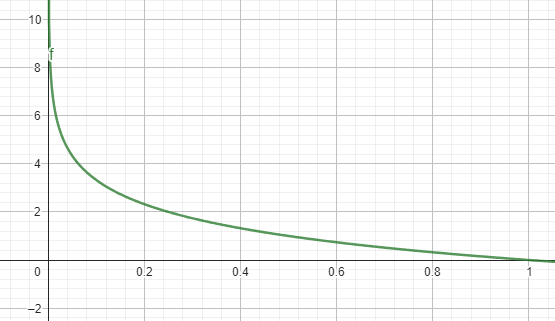
我們先把算式簡化(適用於單一結果正確情況)
y = - \log_2 x
Cross Entropy
交叉熵
y = - \log_2 x
x=0.1 \text{ }
y=3.3\\
x=0.5 \text{ }
y=1.0\\
x=0.8 \text{ }
y=0.32
我們先把算式簡化(適用於單一結果正確情況)
Cross Entropy
交叉熵
y = - \log_2 x
x=0.1 \text{ }
y=3.3\\
x=0.5 \text{ }
y=1.0\\
x=0.8 \text{ }
y=0.32
代表著當x的比例越低 數值越高
我們先把算式簡化(適用於單一結果正確情況)
Cross Entropy
交叉熵
Cross Entropy
交叉熵
當預測值偏離1(正確)越遠,熵增加的越快
所以說我們要讓Loss越低越好
Cross Entropy
交叉熵
def cross_entropy(self, y_output: np.ndarray, y_label: np.ndarray) -> int:
return -np.dot(y_label, np.log2(y_output))交叉熵
得到了Loss之後
就可以準備來更新參數了
Cross Entropy
def cross_entropy(self, y_output: np.ndarray, y_label: np.ndarray) -> int:
    return -np.dot(y_label, np.log2(y_output))
Optimization
最佳化
我們先將不同的W對應的Loss來作圖
我們先將不同的W對應的Loss來作圖
Loss
W
我們要做的就是找到圖中Loss最低點
並將W更新
Loss
W
我們要做的就是找到圖中Loss最低點
並將W更新
問題是要怎麼讓程式知道最低點呢?
Loss
W
直接把每個組合試過一遍
Loss
W
Loss
W
Loss
W
Loss
W
直接把每個組合試過一遍
各位競程大師用腳想都知道那個時間複雜度會爆炸
Loss
W
Loss
W
Loss
W
Loss
W
況且我們還不只一個參數
Gradient Descent
梯度下降
Gradient Descent
x^{t+1} = x^t - \gamma \nabla f(x^t)
梯度下降
Gradient Descent
x^{t+1} = x^t - \gamma \nabla f(x^t)
梯度下降
看起來很難懂
Gradient Descent
x^{t+1} = x^t - \gamma \nabla f(x^t)
梯度下降
看起來很難懂
直接上圖
Gradient Descent
梯度下降
Loss
W
Gradient Descent
梯度下降
Loss
W
目標點
Gradient Descent
梯度下降
Loss
W
起始點
Gradient Descent
梯度下降
Loss
W
起始點
對起始點做微分
Loss
W
對起始點做微分
從微分後得到的斜率就可以判斷低點是在左邊還是右邊
Loss
W
對起始點做微分
從微分後得到的斜率就可以判斷低點是在左邊還是右邊
Loss
W
對起始點做微分
從微分後得到的斜率就可以判斷低點是在左邊還是右邊
Loss
W
對起始點做微分
從微分後得到的斜率就可以判斷低點是在左邊還是右邊
並且向那個方向前進直到斜率=0
Loss
W
對起始點做微分
從微分後得到的斜率就可以判斷低點是在左邊還是右邊
並且向那個方向前進直到斜率=0
x^{t+1} = x^t - \gamma \nabla f(x^t)
但是我們的參數顯然不是只有一個
所以要對每個參數分別進行偏微分
x^{t+1} = x^t - \gamma \nabla f(x^t)
x^{t+1} = x^t - \gamma \nabla f(x^t)
下一次的位置
x^{t+1} = x^t - \gamma \nabla f(x^t)
下一次的位置
這次的位置
x^{t+1} = x^t - \gamma \nabla f(x^t)
下一次的位置
這次的位置
學習率
x^{t+1} = x^t - \gamma \nabla f(x^t)
下一次的位置
這次的位置
學習率
偏微分
梯度下降會產生的問題
x^{t+1} = x^t - \gamma \nabla f(x^t)

Plateaus
Exploding Gradients
Saddle Points
Local Minima
Oscillations
Vanishing Gradients
Local Minima
局部最小值
有機率找到的不是全域最小值
而是局部最小值
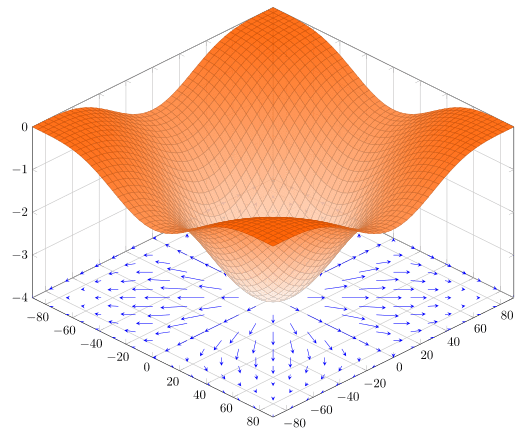
Saddle Points
鞍點
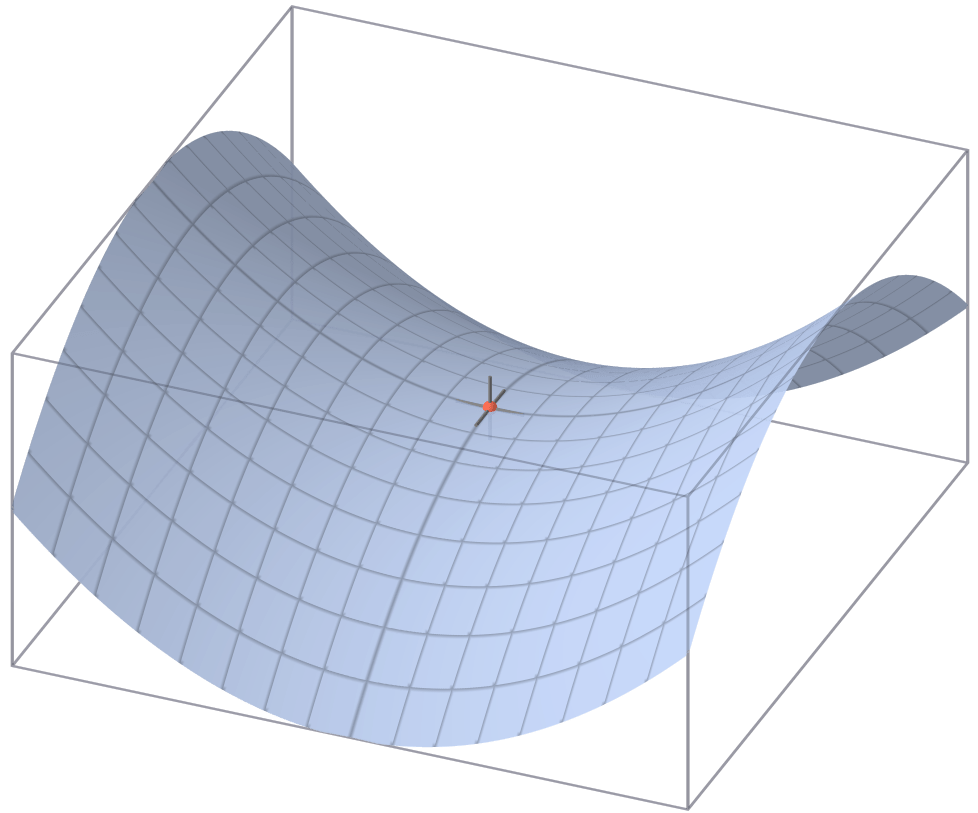
長得像鞍一樣的形狀
若是結果趨近於這種形狀
將會產生其中一軸最低點
=另一軸最高點
在梯度下降時便會容易卡在裡面
Plateaus
高原 (?
如果一部份的路徑過於平緩可能會
導致梯度下降的速度變很慢
Oscillations
震盪
當學習率過高時有可能一直卡在一個谷中找不到最低點
Vanishing Gradients
梯度消失
反向傳播時重複對梯度做微分後的activation function
有時候會造成梯度快速減少最終消失
x^{t+1} = x^t - \gamma \nabla f(x^t)
舉個例子
Sigmoid在微分過後函數落在[1/4, 0]之區間
若重複進行便有可能會使梯度趨近於0
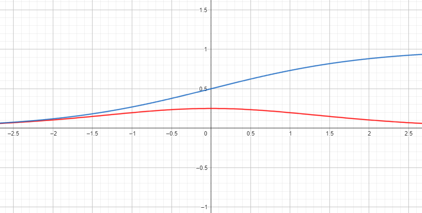
Sigmoid
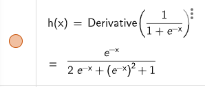
藍線: 原
紅線: 微分後
Exploding Gradients
梯度爆炸
Exploding Gradients
梯度爆炸
同理於梯度消失
當梯度不斷變大之後會發生超過程式上限的狀況
最終會導致bug
Backpropagation
反向傳播
先來固定等一下用的符號
z^{(n)}_0
z^{(n)}_1
z^{(n)}_2
z^{(n-1)}_0
z^{(n-1)}_1
\hat y
L
以z表示該神經元過激勵函數前的輸出
以y表示神經網路的輸出
以L表示Loss
w_{i}^{(n)}(grad)
先來假設現在要求某個w的梯度
Loss
W
w_{i}^{(n)}(grad) =
\frac{\partial L}{\partial w_i^{(n)}}
\frac{\partial L}{\partial w_i^{(n)}}
= \frac{\partial L}{\partial z_i^{(n)}} \cdot
\frac{\partial z_i^{(n)}}{\partial w_i^{(n)}}
該w的梯度為在整個產生Loss的函式中對w微分的結果
w_{i}^{(n)}(grad) =
\frac{\partial L}{\partial w_i^{(n)}}
\frac{\partial L}{\partial w_i^{(n)}}
= \frac{\partial L}{\partial z_i^{(n)}} \cdot
\frac{\partial z_i^{(n)}}{\partial w_i^{(n)}}
該w的梯度為在整個產生Loss的函式中對w微分的結果
我們先來求在該神經元中對w微分
->
\hat y
->
L
z^{(0)}_0
z^{(0)}_1
z^{(1)}_0
z^{(1)}_1
z^{(1)}_2
->
\hat y
->
L
z^{(0)}_0
z^{(0)}_1
z^{(1)}_0
z^{(1)}_1
z^{(1)}_2
w_0
->
\hat y
->
L
z^{(0)}_0
z^{(0)}_1
z^{(1)}_0
z^{(1)}_1
z^{(1)}_2
w_0
w_1
\frac{\partial z_0^{(1)}}{\partial w_0} = a_0^{(0)}
z_0^{(1)} = w_0a_0^{(0)} +
w_1a_1^{(0)} +
b
\frac{\partial z_0^{(1)}}{\partial w_1} = a_1^{(0)}
a_0^{(0)} = \sigma(z_0^{(0)})
z^{(0)}_0
z^{(0)}_1
z^{(1)}_0
z^{(1)}_1
z^{(1)}_2
w_0
a_0^{(0)}
a_1^{(0)}
w_1
這邊的算式可得知欲求之值之後其實就是前一項的a
(a亦為乘上權重前的參數)
w_{i}^{(n)}(grad) =
\frac{\partial L}{\partial w_i^{(n)}}
\frac{\partial L}{\partial w_i^{(n)}}
= \frac{\partial L}{\partial z_i^{(n)}} \cdot
\frac{\partial z_i^{(n)}}{\partial w_i^{(n)}}
回到這一頁
w_{i}^{(n)}(grad) =
\frac{\partial L}{\partial w_i^{(n)}}
\frac{\partial L}{\partial w_i^{(n)}}
= \frac{\partial L}{\partial z_i^{(n)}} \cdot
\frac{\partial z_i^{(n)}}{\partial w_i^{(n)}}
接下來求整個函式中對該神經元的微分
\frac{\partial L}{\partial z_0^{(0)}}
=
\frac{\partial a}{\partial z_0^{(0)}}
\frac{\partial L}{\partial a}
a = \sigma(z_0^{(0)})
\frac{\partial L}{\partial a}
=
\frac{\partial z_0^{(1)}}{\partial a}
\frac{\partial L}{\partial z_0^{(1)}}
+
\frac{\partial z_1^{(1)}}{\partial a}
\frac{\partial L}{\partial z_1^{(1)}}
\frac{\partial L}{\partial z_0^{(0)}}
=
\sigma^{\prime}(z_0^{(0)})[
w_1 \frac{\partial L}{\partial z_0^{(1)}}
+
w_2 \frac{\partial L}{\partial z_1^{(1)}}
]
w_0
w_1
z^{(0)}_0
z^{(0)}_1
z^{(1)}_0
z^{(1)}_1
a
\frac{\partial L}{\partial z_0^{(0)}}
=
\frac{\partial a}{\partial z_0^{(0)}}
\frac{\partial L}{\partial a}
a = \sigma(z_0^{(0)})
\frac{\partial L}{\partial a}
=
\frac{\partial z_0^{(1)}}{\partial a}
\frac{\partial L}{\partial z_0^{(1)}}
+
\frac{\partial z_1^{(1)}}{\partial a}
\frac{\partial L}{\partial z_1^{(1)}}
\frac{\partial L}{\partial z_0^{(0)}}
=
\sigma^{\prime}(z_0^{(0)})[
w_0 \frac{\partial L}{\partial z_0^{(1)}}
+
w_1 \frac{\partial L}{\partial z_1^{(1)}}
]
w_0
w_1
z^{(0)}_0
z^{(0)}_1
z^{(1)}_0
z^{(1)}_1
a
這邊可以發現說其實我們可以藉由這個遞迴關係直接拿最後面的資訊往前算
至於最後面的資訊....
根據選用的loss function不同計算也會不一樣
如果是範例中的softmax + cross entropy的話
微分過後會變成
y_i - t_i
w_{i}^{(n)}(grad) =
\frac{\partial L}{\partial w_i^{(n)}}
\frac{\partial L}{\partial w_i^{(n)}}
= \frac{\partial L}{\partial z_i^{(n)}} \cdot
\frac{\partial z_i^{(n)}}{\partial w_i^{(n)}}
由此可知先記錄一開始向前傳播時拿到的資訊(z)後
從後方再進行一次傳播便可獲得每個參數的梯度
->
\hat y
->
L
z^{(0)}_0
z^{(0)}_1
z^{(1)}_0
z^{(1)}_1
z^{(1)}_2
統整一下整個神經網路的最佳化流程
->
\hat y
->
L
z^{(0)}_0
z^{(0)}_1
z^{(1)}_0
z^{(1)}_1
z^{(1)}_2
資訊傳入
->
\hat y
->
L
z^{(0)}_0
z^{(0)}_1
z^{(1)}_0
z^{(1)}_1
z^{(1)}_2
過神經網路運算
->
\hat y
->
L
z^{(0)}_0
z^{(0)}_1
z^{(1)}_0
z^{(1)}_1
z^{(1)}_2
得到結果與Loss
<-
\hat y
<-
L
z^{(0)}_0
z^{(0)}_1
z^{(1)}_0
z^{(1)}_1
z^{(1)}_2
從結果計算反向傳播時的輸入
<-
\hat y
<-
L
z^{(0)}_0
z^{(0)}_1
z^{(1)}_0
z^{(1)}_1
z^{(1)}_2
更新參數
<-
\hat y
<-
L
z^{(0)}_0
z^{(0)}_1
z^{(1)}_0
z^{(1)}_1
z^{(1)}_2
更新參數完畢
b_{i}^{(n)}(grad) =
\frac{\partial L}{\partial b_i^{(n)}}
\frac{\partial L}{\partial b_i^{(n)}}
= \frac{\partial L}{\partial z_i^{(n)}} \cdot
\frac{\partial z_i^{(n)}}{\partial b_i^{(n)}}
最後補充一下b的部分
\frac{\partial L}{\partial z_i^{(n)}}
= \text{同$w$情況}
\frac{\partial z_i^{(n)}}{\partial b_i^{(n)}}
= 1
z_0^{(1)} = w_1z_0^{(0)} +
w_2z_1^{(0)} + \cdots +
b
Programing
編程
記得先匯入需要的函式庫
pip install numpy
pip install matplotlib
pip install keras
pip install tensorflow
numpy:提供矩陣功能
matplotlib:繪製圖表使用
keras&tensorflow:提供MNIST資料庫
MNIST數據集:一堆手寫數字圖片的數據集
常被用於人工智慧測試辨識數字使用
先設定好 activation functions
# act.py
import numpy as np

def relu(x):
    return np.maximum(0, x)

def drelu(x):
    return np.where(x > 0, 1, 0)
np.maximum(a, x)
相當於對陣列內每個元素取 max(a, x)
np.where(condition, a, b)
會將x的每一項使用參數中的判斷式做判斷
根據 true or false 會將輸出陣列的那一項
設定為a or b
事前準備完成後就可以來刻神經網路了
事前準備完成後就可以來刻神經網路了
第一步先來初始化一個神經網路的物件
class NeuralNetwork:
    def __init__(self, layers: list[int], activation_function: Callable, dactivation_function: Callable=None, learning_rate: float=1e-3) -> None:
        self.layers = layers
        self.learning_rate = learning_rate
        self.act = activation_function
        self.dact = dactivation_function or self.d(activation_function)
        self.delta = 1e-10
        self.Z: list[np.ndarray] = [np.zeros(layers[0])]
        self.W: list[np.ndarray] = [np.zeros(layers[0])]
        self.B: list[np.ndarray] = [np.zeros(layers[0])]
        self.output: list[np.ndarray]  = [np.zeros(layers[0])]

        for i in range(1, len(self.layers)):
            self.W.append(np.random.randn(self.layers[i], self.layers[i-1]) * np.sqrt(2/layers[i-1]))
            self.B.append(np.zeros(self.layers[i]))
            self.Z.append(np.zeros(self.layers[i]))
            self.output.append(np.zeros(self.layers[i]))


    def d(self, f: Callable) -> Callable:
        delta = 1e-10j
        def df(x): return f(x + delta).imag / delta.imag
        return df
我們希望能夠透過輸入來決定神經網路的結構
e.g. layers = [16, 32, 64, 32, 10]
那麼輸入層 = 16 輸出層 = 10 其他層同理
class NeuralNetwork:
    def __init__(self, layers: list[int], activation_function: Callable, dactivation_function: Callable=None, learning_rate: float=1e-3) -> None:
        self.layers = layers
        self.learning_rate = learning_rate
        self.act = activation_function
        self.dact = dactivation_function or self.d(activation_function)
        self.delta = 1e-10
        self.Z: list[np.ndarray] = [np.zeros(layers[0])]
        self.W: list[np.ndarray] = [np.zeros(layers[0])]
        self.B: list[np.ndarray] = [np.zeros(layers[0])]
        self.output: list[np.ndarray]  = [np.zeros(layers[0])]

        for i in range(1, len(self.layers)):
            self.W.append(np.random.randn(self.layers[i], self.layers[i-1]) * np.sqrt(2/layers[i-1]))
            self.B.append(np.zeros(self.layers[i]))
            self.Z.append(np.zeros(self.layers[i]))
            self.output.append(np.zeros(self.layers[i]))


    def d(self, f: Callable) -> Callable:
        delta = 1e-10j
        def df(x): return f(x + delta).imag / delta.imag
        return df
設定學習率 梯度下降會使用到
class NeuralNetwork:
    def __init__(self, layers: list[int], activation_function: Callable, dactivation_function: Callable=None, learning_rate: float=1e-3) -> None:
        self.layers = layers
        self.learning_rate = learning_rate
        self.act = activation_function
        self.dact = dactivation_function or self.d(activation_function)
        self.delta = 1e-10
        self.Z: list[np.ndarray] = [np.zeros(layers[0])]
        self.W: list[np.ndarray] = [np.zeros(layers[0])]
        self.B: list[np.ndarray] = [np.zeros(layers[0])]
        self.output: list[np.ndarray]  = [np.zeros(layers[0])]

        for i in range(1, len(self.layers)):
            self.W.append(np.random.randn(self.layers[i], self.layers[i-1]) * np.sqrt(2/layers[i-1]))
            self.B.append(np.zeros(self.layers[i]))
            self.Z.append(np.zeros(self.layers[i]))
            self.output.append(np.zeros(self.layers[i]))


    def d(self, f: Callable) -> Callable:
        delta = 1e-10j
        def df(x): return f(x + delta).imag / delta.imag
        return df
設定 activation functions
另外構建了一個函數在未給予dact的情況下自動微分
class NeuralNetwork:
    def __init__(self, layers: list[int], activation_function: Callable, dactivation_function: Callable=None, learning_rate: float=1e-3) -> None:
        self.layers = layers
        self.learning_rate = learning_rate
        self.act = activation_function
        self.dact = dactivation_function or self.d(activation_function)
        self.delta = 1e-10
        self.Z: list[np.ndarray] = [np.zeros(layers[0])]
        self.W: list[np.ndarray] = [np.zeros(layers[0])]
        self.B: list[np.ndarray] = [np.zeros(layers[0])]
        self.output: list[np.ndarray]  = [np.zeros(layers[0])]

        for i in range(1, len(self.layers)):
            self.W.append(np.random.randn(self.layers[i], self.layers[i-1]) * np.sqrt(2/layers[i-1]))
            self.B.append(np.zeros(self.layers[i]))
            self.Z.append(np.zeros(self.layers[i]))
            self.output.append(np.zeros(self.layers[i]))


    def d(self, f: Callable) -> Callable:
        delta = 1e-10j
        def df(x): return f(x + delta).imag / delta.imag
        return df
設定一個很小的數字
用以防止特定地方可能除以0導致程式發生錯誤
class NeuralNetwork:
    def __init__(self, layers: list[int], activation_function: Callable, dactivation_function: Callable=None, learning_rate: float=1e-3) -> None:
        self.layers = layers
        self.learning_rate = learning_rate
        self.act = activation_function
        self.dact = dactivation_function or self.d(activation_function)
        self.delta = 1e-10
        self.Z: list[np.ndarray] = [np.zeros(layers[0])]
        self.W: list[np.ndarray] = [np.zeros(layers[0])]
        self.B: list[np.ndarray] = [np.zeros(layers[0])]
        self.output: list[np.ndarray]  = [np.zeros(layers[0])]

        for i in range(1, len(self.layers)):
            self.W.append(np.random.randn(self.layers[i], self.layers[i-1]) * np.sqrt(2/layers[i-1]))
            self.B.append(np.zeros(self.layers[i]))
            self.Z.append(np.zeros(self.layers[i]))
            self.output.append(np.zeros(self.layers[i]))


    def d(self, f: Callable) -> Callable:
        delta = 1e-10j
        def df(x): return f(x + delta).imag / delta.imag
        return df
建立存放參數的陣列
並且事先以填充0初始化每個神經元的參數陣列大小
class NeuralNetwork:
    def __init__(self, layers: list[int], activation_function: Callable, dactivation_function: Callable=None, learning_rate: float=1e-3) -> None:
        self.layers = layers
        self.learning_rate = learning_rate
        self.act = activation_function
        self.dact = dactivation_function or self.d(activation_function)
        self.delta = 1e-10
        self.Z: list[np.ndarray] = [np.zeros(layers[0])]
        self.W: list[np.ndarray] = [np.zeros(layers[0])]
        self.B: list[np.ndarray] = [np.zeros(layers[0])]
        self.output: list[np.ndarray]  = [np.zeros(layers[0])]

        for i in range(1, len(self.layers)):
            self.W.append(np.random.randn(self.layers[i], self.layers[i-1]) * np.sqrt(2/layers[i-1]))
            self.B.append(np.zeros(self.layers[i]))
            self.Z.append(np.zeros(self.layers[i]))
            self.output.append(np.zeros(self.layers[i]))


    def d(self, f: Callable) -> Callable:
        delta = 1e-10j
        def df(x): return f(x + delta).imag / delta.imag
        return df
使用 Kaiming Initialization
詳細說明礙於篇幅問題此處不過多著墨
def softmax(self, x):
  exp_x = np.exp(x - np.max(x))
  return exp_x / np.sum(exp_x)


def cross_entropy(self, y: np.ndarray) -> np.float64:
  return -np.dot(y.T, np.log(self.output[-1] + self.delta))
在物件內建立好待會會使用到的算式
另外前面提到的delta在cross entropy時便使用到了
np.dot(x, y)
內積 詳細可見線性代數章節
np.exp(x)
對每個x的元素取 e^x
def save_params(self, filename: str="params.json"):
    with open(filename, "w") as f:
		json.dump({"W": self.W, "B": self.B}, f, indent=4, cls=NumpyArrayEncoder)


def load_params(self, filename: str="params.json"):
	with open(filename, "r") as f:
		params = json.load(f)
		self.W = []
		self.B = []
		for w in params["W"]: self.W.append(np.asarray(w))
		for b in params["B"]: self.B.append(np.asarray(b))
設定個儲存參數的東西
可以避免每次都要重複花時間去訓練
另外由於 numpy array 無法被 json 序列化
因此需要使用自訂的 encoder
# encoder.py
import json
import numpy as np

class NumpyArrayEncoder(json.JSONEncoder):
    def default(self, obj):
        if isinstance(obj, np.ndarray):
            return obj.tolist()
        return json.JSONEncoder.default(self, obj)
另外由於 numpy array 無法被 json 序列化
因此需要使用自訂的 encoder
自訂 encoder 會將物件內的每個 numpy array
進行 tolist() 操作
讓他可以變成 python 內建的 list 被儲存到 json
def forward(self, x: np.ndarray) -> np.ndarray:
    assert x.shape[0] == self.layers[0]
    self.output[0] = x

    for i in range(1, len(self.layers)):
        self.Z[i] = np.dot(self.W[i], self.output[i-1]) + self.B[i]
        if i == len(self.layers)-1: self.output[i] = self.softmax(self.Z[i])
        else: self.output[i] = self.act(self.Z[i])

    return self.output[-1]
前向傳播 啟動
def forward(self, x: np.ndarray) -> np.ndarray:
    assert x.shape[0] == self.layers[0]
    self.output[0] = x

    for i in range(1, len(self.layers)):
        self.Z[i] = np.dot(self.W[i], self.output[i-1]) + self.B[i]
        if i == len(self.layers)-1: self.output[i] = self.softmax(self.Z[i])
        else: self.output[i] = self.act(self.Z[i])

    return self.output[-1]
\vec Z = \vec X \cdot \vec W + \vec B
\vec{\mathtt{output}}_i = \sigma(\vec Z) \\
\vec{\mathtt{output}}_n = \sigma_{softmax}(\vec Z)
def backward(self, y: np.ndarray) -> None:
    x = self.output[-1] - y

    for i in range(len(self.layers)-1, 0, -1):
        t = x * self.dact(self.Z[i])
        x = np.dot(self.W[i].T, t)
        self.W[i] -= self.learning_rate * np.outer(t, self.output[i-1])
        self.B[i] -= self.learning_rate * t
反向傳播 啟動
def backward(self, y: np.ndarray) -> None:
    x = self.output[-1] - y

    for i in range(len(self.layers)-1, 0, -1):
        t = x * self.dact(self.Z[i])
        x = np.dot(self.W[i].T, t)
        self.W[i] -= self.learning_rate * np.outer(t, self.output[i-1])
        self.B[i] -= self.learning_rate * t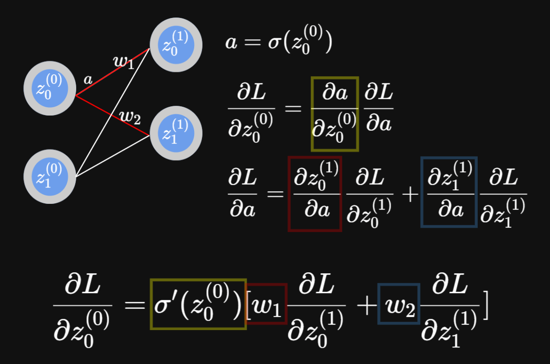
def backward(self, y: np.ndarray) -> None:
x = self.output[-1] - y
for i in range(len(self.layers)-1, 0, -1):
t = x * self.dact(self.Z[i])
x = np.dot(self.W[i].T, t)
self.W[i] -= self.learning_rate * np.outer(t, self.output[i-1])
self.B[i] -= self.learning_rate * tdef backward(self, y: np.ndarray) -> None:
x = self.output[-1] - y
for i in range(len(self.layers)-1, 0, -1):
t = x * self.dact(self.Z[i])
x = np.dot(self.W[i].T, t)
self.W[i] -= self.learning_rate * np.outer(t, self.output[i-1])
self.B[i] -= self.learning_rate * tdef backward(self, y: np.ndarray) -> None:
x = self.output[-1] - y
for i in range(len(self.layers)-1, 0, -1):
t = x * self.dact(self.Z[i])
x = np.dot(self.W[i].T, t)
self.W[i] -= self.learning_rate * np.outer(t, self.output[i-1])
self.B[i] -= self.learning_rate * t將反向傳播得到的資訊
乘上權重
def backward(self, y: np.ndarray) -> None:
    x = self.output[-1] - y

    for i in range(len(self.layers)-1, 0, -1):
        t = x * self.dact(self.Z[i])
        x = np.dot(self.W[i].T, t)
        self.W[i] -= self.learning_rate * np.outer(t, self.output[i-1])
        self.B[i] -= self.learning_rate * t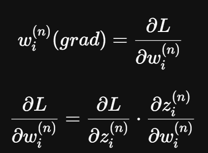
\frac{\partial z_i^{(n)}}{\partial w_i^{(n)}} = \sigma(z_i^{(n-1)})
\frac{\partial z_i^{(n)}}{\partial b_i^{(n)}} = 1
def backward(self, y: np.ndarray) -> None:
    x = self.output[-1] - y

    for i in range(len(self.layers)-1, 0, -1):
        t = x * self.dact(self.Z[i])
        x = np.dot(self.W[i].T, t)
        self.W[i] -= self.learning_rate * np.outer(t, self.output[i-1])
self.B[i] -= self.learning_rate * t\frac{\partial z_i^{(n)}}{\partial w_i^{(n)}} = \sigma(z_i^{(n-1)})
\frac{\partial z_i^{(n)}}{\partial b_i^{(n)}} = 1
因此w要多乘一個過未經微分的sigmoid的x
def fit(self, x: np.ndarray, y: np.ndarray) -> np.float64:
self.forward(x)
loss = self.cross_entropy(y)
self.backward(y)
return loss每次進行一次最佳化就
過一次正向傳播計算loss後
進行反向傳播更新參數
完整Code
# act.py
import numpy as np
def relu(x):
return np.maximum(0, x)
def drelu(x):
return np.where(x > 0, 1, 0)# *)#$#*)%*)#$#)*%
完整Code
# encoder.py
import json
import numpy as np
class NumpyArrayEncoder(json.JSONEncoder):
def default(self, obj):
if isinstance(obj, np.ndarray):
return obj.tolist()
return json.JSONEncoder.default(self, obj)# *)#$#*)%*)#$#)*%
完整Code
# nn.py
import numpy as np
import json
from typing import Callable
from encoder import NumpyArrayEncoder
class NeuralNetwork:
def __init__(self, layers: list[int], activation_function: Callable, dactivation_function: Callable=None, learning_rate: float=1e-3) -> None:
self.layers = layers
self.learning_rate = learning_rate
self.act = activation_function
self.dact = dactivation_function or self.d(activation_function)
self.delta = 1e-10
self.Z: list[np.ndarray] = [np.zeros(layers[0])]
self.W: list[np.ndarray] = [np.zeros(layers[0])]
self.B: list[np.ndarray] = [np.zeros(layers[0])]
self.output: list[np.ndarray] = [np.zeros(layers[0])]
for i in range(1, len(self.layers)):
self.W.append(np.random.randn(self.layers[i], self.layers[i-1]) * np.sqrt(2/layers[i-1]))
self.B.append(np.zeros(self.layers[i]))
self.Z.append(np.zeros(self.layers[i]))
self.output.append(np.zeros(self.layers[i]))
def d(self, f: Callable) -> Callable:
delta = 1e-10j
def df(x): return f(x + delta).imag / delta.imag
return df
def softmax(self, x):
exp_x = np.exp(x - np.max(x))
return exp_x / np.sum(exp_x)
def cross_entropy(self, y: np.ndarray) -> np.float64:
return -np.dot(y.T, np.log(self.output[-1] + self.delta))
def forward(self, x: np.ndarray) -> np.ndarray:
assert x.shape[0] == self.layers[0]
self.output[0] = x
for i in range(1, len(self.layers)):
self.Z[i] = np.dot(self.W[i], self.output[i-1]) + self.B[i]
if i == len(self.layers)-1: self.output[i] = self.softmax(self.Z[i])
else: self.output[i] = self.act(self.Z[i])
return self.output[-1]
def backward(self, y: np.ndarray) -> None:
    x = self.output[-1] - y

    for i in range(len(self.layers)-1, 0, -1):
        t = x * self.dact(self.Z[i])
        x = np.dot(self.W[i].T, t)
        self.W[i] -= self.learning_rate * np.outer(t, self.output[i-1])
        self.B[i] -= self.learning_rate * t
def fit(self, x: np.ndarray, y: np.ndarray) -> np.float64:
self.forward(x)
loss = self.cross_entropy(y)
self.backward(y)
return loss
def save_params(self, filename: str="params.json"):
with open(filename, "w") as f:
json.dump({"W": self.W, "B": self.B}, f, indent=4, cls=NumpyArrayEncoder)
def load_params(self, filename: str="params.json"):
with open(filename, "r") as f:
params = json.load(f)
self.W = []
self.B = []
for w in params["W"]: self.W.append(np.asarray(w))
for b in params["B"]: self.B.append(np.asarray(b))# *)#$#*)%*)#$#)*%
Training
訓練
我們期望運行神經網路的流程如下
訓練神經網路 => 測試模型準確率
也就是說我們的啟動檔案
會匯入模型以及MNIST
並且進行訓練與測試
最後會得到準確率的結果與過程的loss變化
建立一個 main.py
此時檔案結構應如下
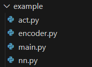
接著來編寫 main.py
import numpy as np
import matplotlib.pyplot as plt
from keras.datasets import mnist
from nn import NeuralNetwork
from act import relu, drelu先引入所需函式庫
learning_rate = 1e-3
data_size = 784
batch_size = 64
max_trains = 50000
epochs = 3
save = True設定參數
learning_rate: 學習率
data_size: 資料大小(等同輸入層的層數)
batch_size: 每次訓練並輸出的批次量
max_trains: 最大訓練次數
epochs: 總共訓練幾個epoch
save: 是否要儲存參數
(x_train_image, y_train_label), (x_test_image, y_test_label) = mnist.load_data()
x_trains = np.array(x_train_image).reshape(len(x_train_image), 784).astype("float64")/255
x_tests = np.array(x_test_image).reshape(len(x_test_image), 784).astype("float64")/255
y_trains = np.eye(10)[y_train_label]
y_tests = np.eye(10)[y_test_label]從MNIST中載入資料
並且將圖片轉換成一維陣列後設定型別
除以255是為了讓灰階區間從[0, 255]->[0, 1]
(x_train_image, y_train_label), (x_test_image, y_test_label) = mnist.load_data()
x_trains = np.array(x_train_image).reshape(len(x_train_image), 784).astype("float64")/255
x_tests = np.array(x_test_image).reshape(len(x_test_image), 784).astype("float64")/255
y_trains = np.eye(10)[y_train_label]
y_tests = np.eye(10)[y_test_label]np.eye(n)會建立一個n*n的單位矩陣
np.eye(3) =
\left[
\begin{matrix}
1 & 0 & 0 \\
0 & 1 & 0 \\
0 & 0 & 1
\end{matrix}
\right]
(x_train_image, y_train_label), (x_test_image, y_test_label) = mnist.load_data()
x_trains = np.array(x_train_image).reshape(len(x_train_image), 784).astype("float64")/255
x_tests = np.array(x_test_image).reshape(len(x_test_image), 784).astype("float64")/255
y_trains = np.eye(10)[y_train_label]
y_tests = np.eye(10)[y_test_label]那為什麼要這麼做呢
因為我們要讓label的形式轉換一下
3 \rightarrow
\left[
\begin{matrix}
0&0&0&1&0&
0&0&0&0&0
\end{matrix}
\right]
※它給的label是0-based 不用減一
nn = NeuralNetwork(layers=[784, 256, 128, 64, 10], activation_function=relu, dactivation_function=drelu, learning_rate=learning_rate)
train_loss = nn.train(x_trains, y_trains, epochs, batch_size, max_trains, save)
test_loss = nn.predict(x_tests, y_tests)創建神經網路物件
並依序從訓練及預測函式拿到loss
(函式內容會在後面章節提到)
plt.plot(train_loss, label="Train Loss")
plt.xlabel("Epoch")
plt.ylabel("Loss")
plt.legend()
plt.show()使用matplotlib函式庫繪製loss的變化圖表
完整Code
# main.py
import numpy as np
import matplotlib.pyplot as plt
from keras.datasets import mnist
from nn import NeuralNetwork
from act import relu, drelu
learning_rate = 1e-3
data_size = 784
batch_size = 64
max_trains = 50000
epochs = 3
save = True
(x_train_image, y_train_label), (x_test_image, y_test_label) = mnist.load_data()
x_trains = np.array(x_train_image).reshape(len(x_train_image), 784).astype("float64")/255
x_tests = np.array(x_test_image).reshape(len(x_test_image), 784).astype("float64")/255
y_trains = np.eye(10)[y_train_label]
y_tests = np.eye(10)[y_test_label]
nn = NeuralNetwork(layers=[784, 256, 128, 64, 10], activation_function=relu, dactivation_function=drelu, learning_rate=learning_rate)
train_loss = nn.train(x_trains, y_trains, epochs, batch_size, max_trains, save)
test_loss = nn.predict(x_tests, y_tests)
plt.plot(train_loss, label="Train Loss")
plt.xlabel("Epoch")
plt.ylabel("Loss")
plt.legend()
plt.show()# *)#$#*)%*)#$#)*%
接著來處理訓練(train)跟預測(predict)的函式
訓練
為了讓每次訓練的輸出
不要因為單次的偏差而顯得數據差過大
我們通常會以一個批次(batch)為單位去做訓練
而批次的大小
訓練
而訓練也可以藉由重複訓練來加強參數
每個epoch便是將整個數據集訓練一遍
而epoch的次數越高 訓練時長越高
但相對的準確率就會提高
另外
最大訓練次數純粹是因為我懶得訓練太久而強制中止的東東
def train(self, x_trains: np.ndarray, y_trains: np.ndarray, epochs: int, batch_size: int=64, max_trains: int=60000, save: bool=False) -> list[np.float64]:
train_loss = []
for epoch in range(epochs):
max_trains = min(max_trains, len(x_trains))
batch_loss = 0
for i in range(0, max_trains, batch_size):
x_batch = x_trains[i:i + batch_size]
y_batch = y_trains[i:i + batch_size]
for x_train, y_train in zip(x_batch, y_batch):
batch_loss += self.fit(x_train, y_train)
print(f"Batch {i//batch_size+1}/{max_trains//batch_size+1}, Loss: {batch_loss/(i+1)}")
avg_loss = batch_loss / max_trains
train_loss.append(avg_loss)
if save:
self.save_params()
print(f"Epoch {epoch+1}/{epochs}, Loss: {avg_loss}, Save: {save}")
return train_loss預測
幾乎同訓練
不過不會更新參數
並且加上準確率
def predict(self, x_tests: np.ndarray, y_tests: np.ndarray) -> list[np.float64]:
test_loss = []
accuracy = 0
for i, (x_test, y_test) in enumerate(zip(x_tests, y_tests)):
output = self.forward(x_test)
loss = self.cross_entropy(y_test)
correct = output.argmax() == y_test.argmax()
if correct:
accuracy += 1
test_loss.append(loss)
print(f"Test Data: {i+1}/{len(x_tests)}, Loss: {loss}, Correct: {correct}")
print(f"Average test loss: {sum(test_loss) / len(test_loss)}")
print(f"Accuracy: {accuracy / len(x_tests)}")
return test_loss完整Code
# nn.py
import numpy as np
import json
from typing import Callable
from encoder import NumpyArrayEncoder
class NeuralNetwork:
def __init__(self, layers: list[int], activation_function: Callable, dactivation_function: Callable=None, learning_rate: float=1e-3) -> None:
self.layers = layers
self.learning_rate = learning_rate
self.act = activation_function
self.dact = dactivation_function or self.d(activation_function)
self.delta = 1e-10
self.Z: list[np.ndarray] = [np.zeros(layers[0])]
self.W: list[np.ndarray] = [np.zeros(layers[0])]
self.B: list[np.ndarray] = [np.zeros(layers[0])]
self.output: list[np.ndarray] = [np.zeros(layers[0])]
for i in range(1, len(self.layers)):
self.W.append(np.random.randn(self.layers[i], self.layers[i-1]) * np.sqrt(2/layers[i-1]))
self.B.append(np.zeros(self.layers[i]))
self.Z.append(np.zeros(self.layers[i]))
self.output.append(np.zeros(self.layers[i]))
def d(self, f: Callable) -> Callable:
delta = 1e-10j
def df(x): return f(x + delta).imag / delta.imag
return df
def softmax(self, x):
exp_x = np.exp(x - np.max(x))
return exp_x / np.sum(exp_x)
def cross_entropy(self, y: np.ndarray) -> np.float64:
return -np.dot(y.T, np.log(self.output[-1] + self.delta))
def forward(self, x: np.ndarray) -> np.ndarray:
assert x.shape[0] == self.layers[0]
self.output[0] = x
for i in range(1, len(self.layers)):
self.Z[i] = np.dot(self.W[i], self.output[i-1]) + self.B[i]
if i == len(self.layers)-1: self.output[i] = self.softmax(self.Z[i])
else: self.output[i] = self.act(self.Z[i])
return self.output[-1]
def backward(self, y: np.ndarray) -> None:
    x = self.output[-1] - y

    for i in range(len(self.layers)-1, 0, -1):
        t = x * self.dact(self.Z[i])
        x = np.dot(self.W[i].T, t)
        self.W[i] -= self.learning_rate * np.outer(t, self.output[i-1])
        self.B[i] -= self.learning_rate * t
def fit(self, x: np.ndarray, y: np.ndarray) -> np.float64:
    self.forward(x)
    loss = self.cross_entropy(y)
    self.backward(y)
    return loss
def predict(self, x_tests: np.ndarray, y_tests: np.ndarray) -> list[np.float64]:
    test_loss = []
    accuracy = 0

    for i, (x_test, y_test) in enumerate(zip(x_tests, y_tests)):
        output = self.forward(x_test)
        loss = self.cross_entropy(y_test)
        correct = output.argmax() == y_test.argmax()

        if correct:
            accuracy += 1

        test_loss.append(loss)
        print(f"Test Data: {i+1}/{len(x_tests)}, Loss: {loss}, Correct: {correct}")

    print(f"Average test loss: {sum(test_loss) / len(test_loss)}")
    print(f"Accuracy: {accuracy / len(x_tests)}")

    return test_loss
def train(self, x_trains: np.ndarray, y_trains: np.ndarray, epochs: int, batch_size: int=64, max_trains: int=60000, save: bool=False) -> list[np.float64]:
train_loss = []
for epoch in range(epochs):
max_trains = min(max_trains, len(x_trains))
batch_loss = 0
for i in range(0, max_trains, batch_size):
x_batch = x_trains[i:i + batch_size]
y_batch = y_trains[i:i + batch_size]
for x_train, y_train in zip(x_batch, y_batch):
batch_loss += self.fit(x_train, y_train)
print(f"Batch {i//batch_size+1}/{max_trains//batch_size+1}, Loss: {batch_loss/(i+1)}")
avg_loss = batch_loss / max_trains
train_loss.append(avg_loss)
if save:
self.save_params()
print(f"Epoch {epoch+1}/{epochs}, Loss: {avg_loss}")
return train_loss
def save_params(self, filename: str="params.json"):
with open(filename, "w") as f:
json.dump({"W": self.W, "B": self.B}, f, indent=4, cls=NumpyArrayEncoder)
def load_params(self, filename: str="params.json"):
with open(filename, "r") as f:
params = json.load(f)
self.W = []
self.B = []
for w in params["W"]: self.W.append(np.asarray(w))
for b in params["B"]: self.B.append(np.asarray(b))# *)#$#*)%*)#$#)*%
Problems
問題
運行速率低下
Slow Processing Speed
有人可能會好奇為什麼不連矩陣一起手刻
因為numpy的程式是基於C語言
因此可以有比一般Python程式更快速的運算速度
運行速率低下
Slow Processing Speed
有人可能會好奇為什麼不連矩陣一起手刻
因為numpy的程式是基於C語言
因此可以有比一般Python程式更快速的運算速度
但它還是有個缺點
那就是它是使用CPU在跑
運行速率低下
Slow Processing Speed
讓numpy可以使用GPU跑的函式庫
使用方式就是把原本的
import numpyimport cupy運行速率低下
Slow Processing Speed
缺點是安裝麻煩一點
視情況要根據你的cuda版本安裝不同的函式庫
超參數
Hyper Parameter
所有需要由使用者自行調整的皆為超參數
像是每層的神經元個數、批次大小、學習率等
這些參數在設定時可以參考現有模型的設定
或是網路上的文章教學
拿前人試出的結果總比自己花時間試好 (?
梯度下降那些問題
About Gradient Descent
手寫辨識...?
Handwriting Recognition
你會發現它在辨識不在資料集內的圖片時
表現的成果異常拙劣
手寫辨識...?
Handwriting Recognition
一部份是由於沒給到其他風格的資料
但另一部份是我們的辨識方式
沒有經由特徵的判斷
而是直接根據像素點的位置去做計算
手寫辨識...?
Handwriting Recognition
這要如何改善呢?
手寫辨識...?
Handwriting Recognition
這要如何改善呢?
Convolutional Neural Network
卷積神經網路
手寫辨識...?
Handwriting Recognition
關於更多資訊歡迎報名
IZCC x 建北電資合作的機器學習放課
保證能帶你學會各種更多有關於機器學習的知識
Convolutional Neural Network
卷積神經網路
資源
Resource
課程結束
Copy of 機器學習-聯課ver.
By oct0920
Copy of 機器學習-聯課ver.
使用於 2025 IZCC x Ruby Taiwan x SCINT 聯合公開課程


