


One Fourth Labs
We deliver courseware in AI and related areas
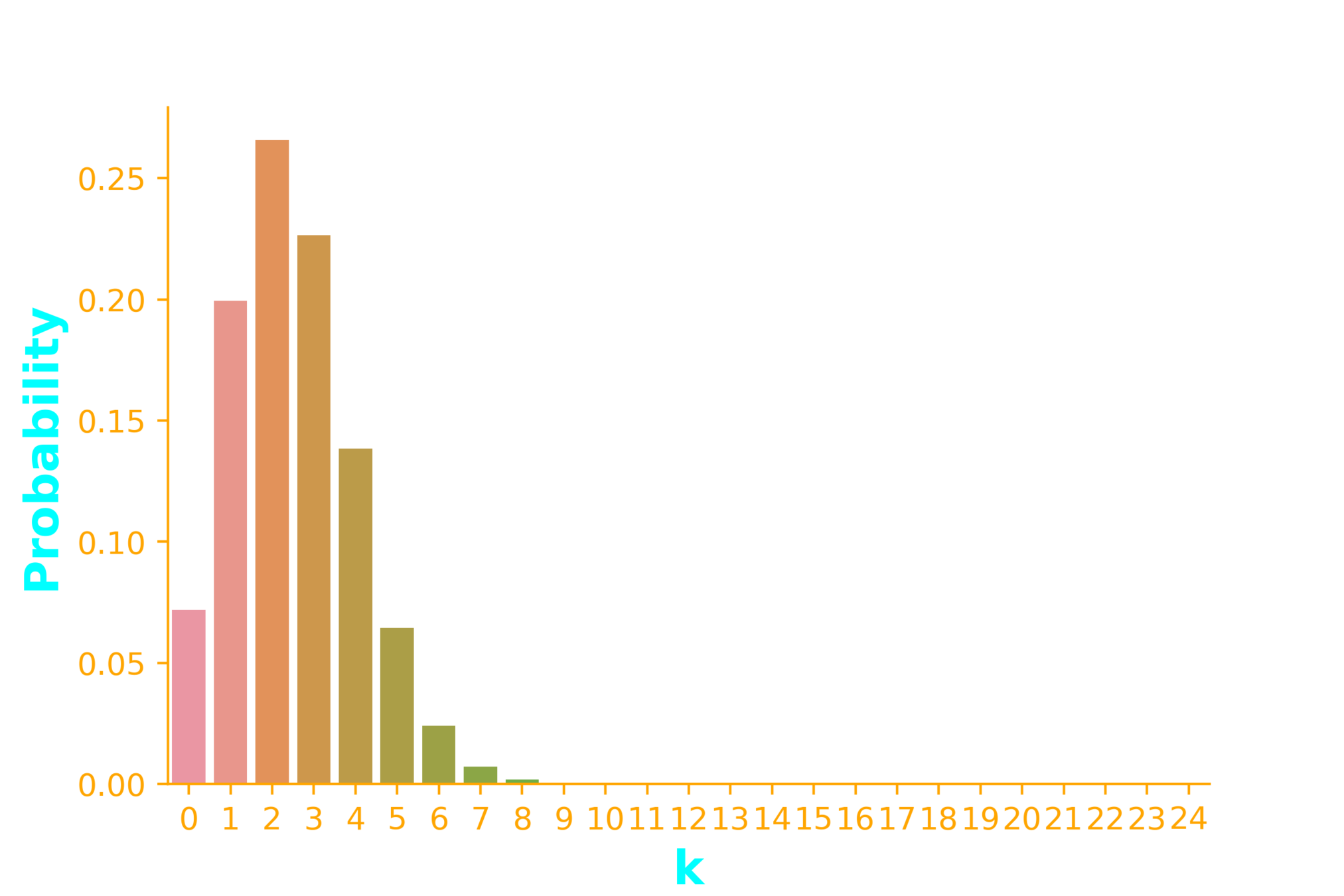
import seaborn as sb
import numpy as np
from scipy.stats import binom

x = np.arange(0, 25)
n=25
p = 0.1

dist = binom(n, p)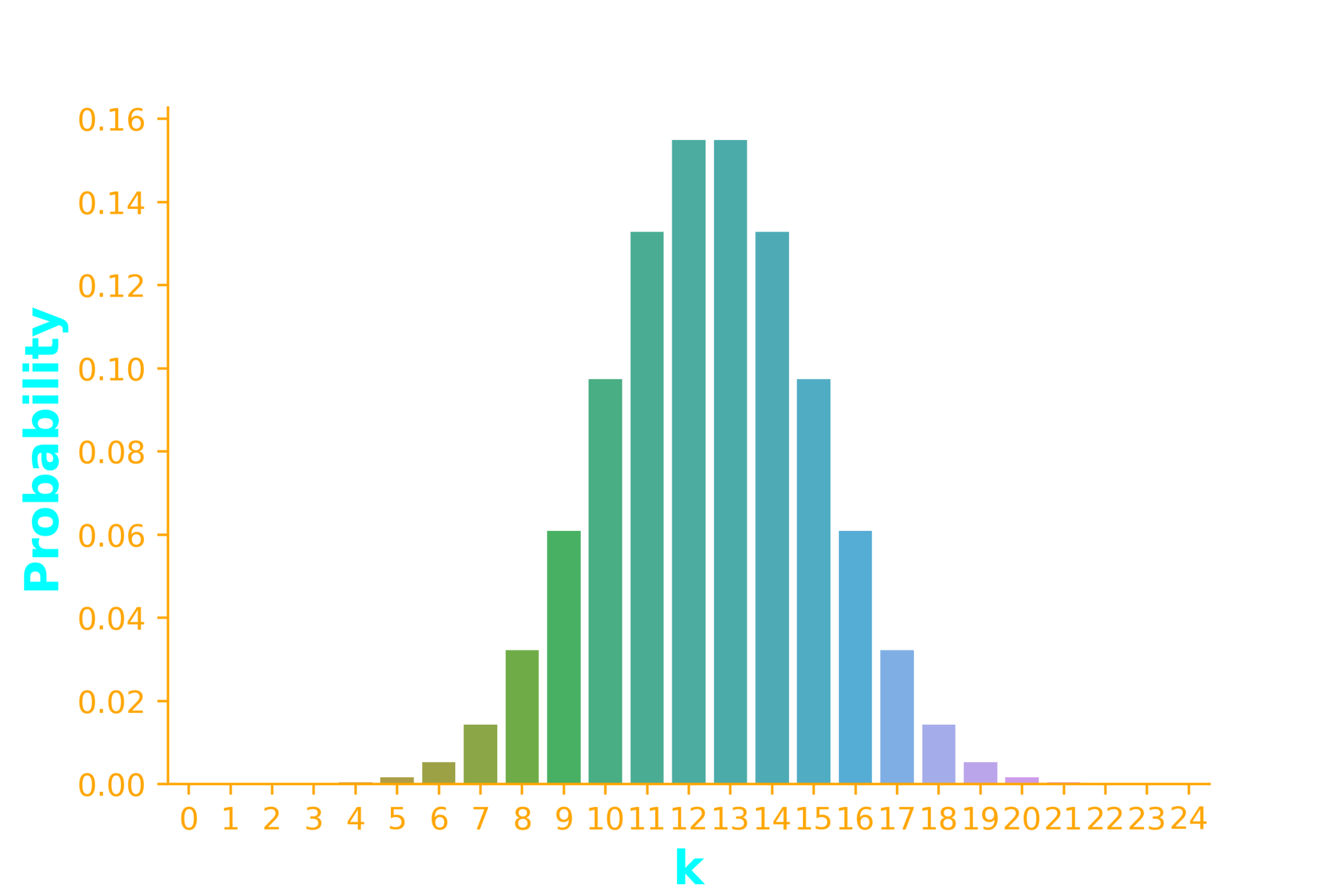
ax = sb.barplot(x=x, y=dist.pmf(x))import seaborn as sb
import numpy as np
from scipy.stats import binom
x = np.arange(0, 25)
n=25
p = 0.1
dist = binom(n, p)
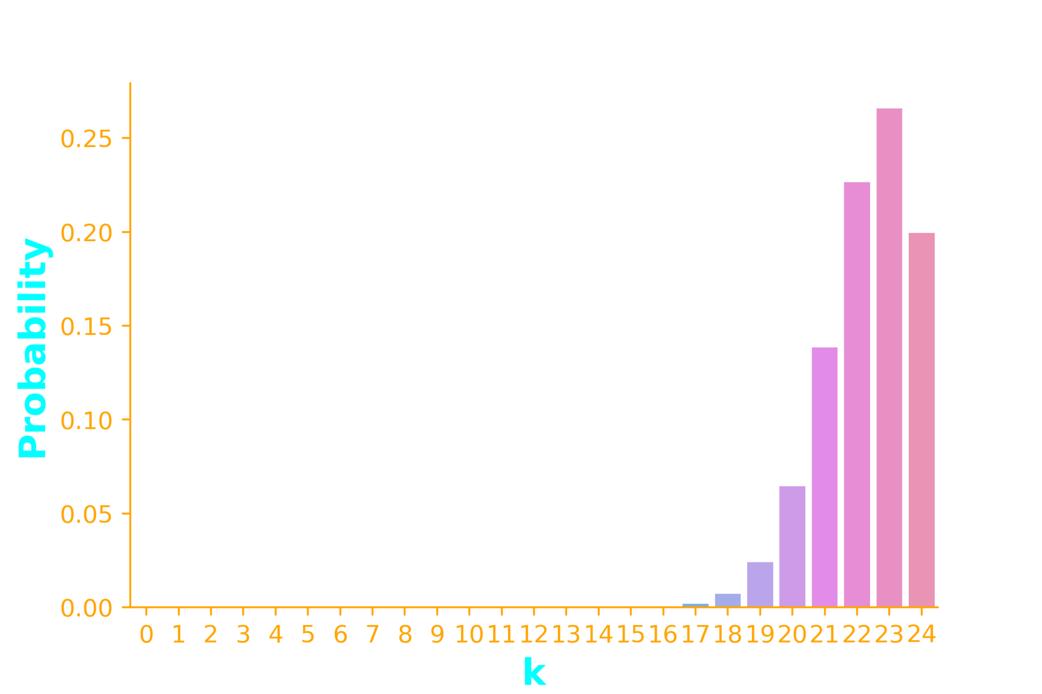
ax = sb.barplot(x=x, y=dist.pmf(x))import seaborn as sb
import numpy as np
from scipy.stats import binom
x = np.arange(0, 25)
n=25
p = 0.1
dist = binom(n, p)
ax = sb.barplot(x=x, y=dist.pmf(x))import seaborn as sb
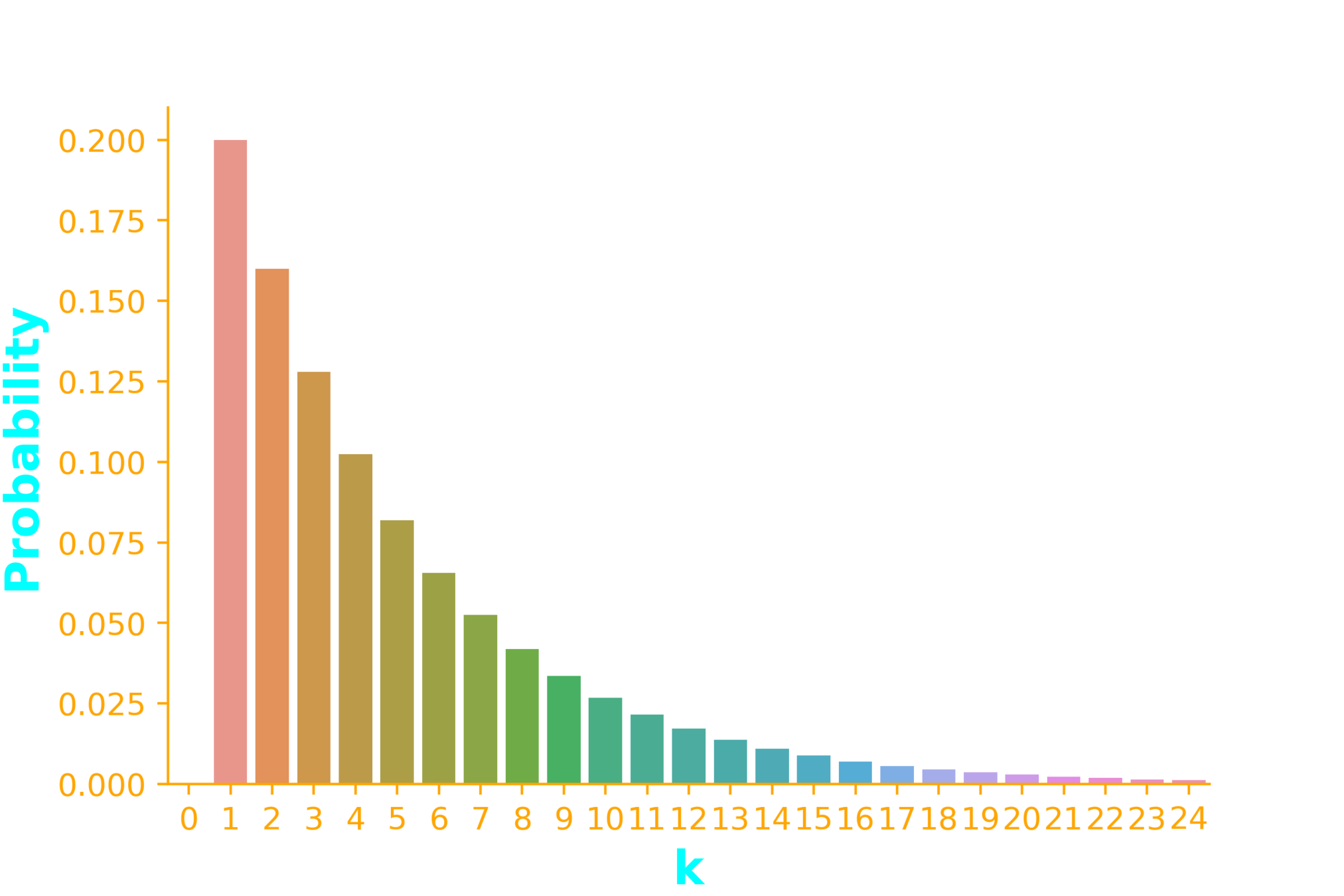
import numpy as np
from scipy.stats import geom
x = np.arange(0, 25)
p = 0.2
dist = geom(p)
ax = sb.barplot(x=x, y=dist.pmf(x))import seaborn as sb
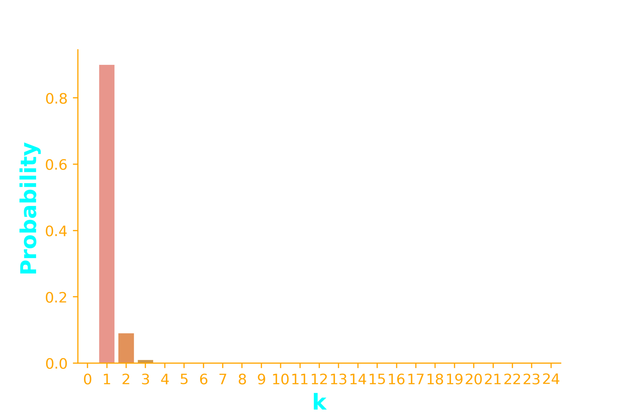
import numpy as np
from scipy.stats import geom
x = np.arange(0, 25)
p = 0.9
dist = geom(p)
ax = sb.barplot(x=x, y=dist.pmf(x))import seaborn as sb
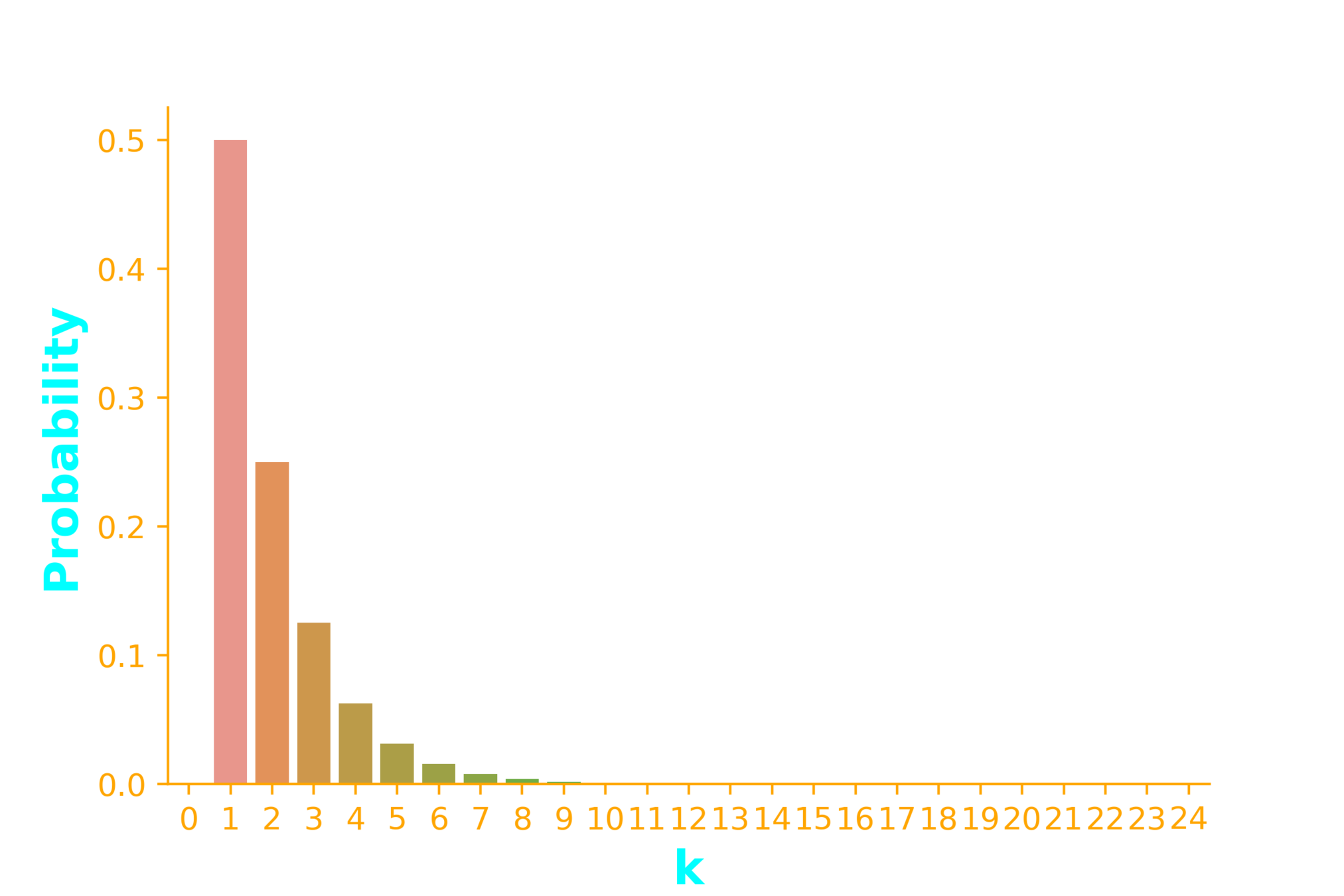
import numpy as np
from scipy.stats import geom
x = np.arange(0, 25)
p = 0.5
dist = geom(p)
ax = sb.barplot(x=x, y=dist.pmf(x))By One Fourth Labs
PadhAI One: FDS Week 3 (MK)


