


orashi
cippus_sss
motivations!
motivations!
History of ML
Interpretability
Flexibility
estimator.fit(Xtrain, ytrain)
estimator.predict(Xtrain, ytrain)
estimator = #@$%&(*param)
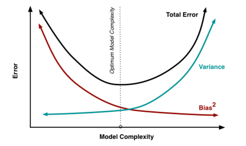
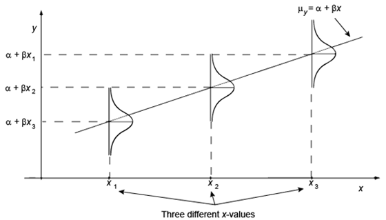
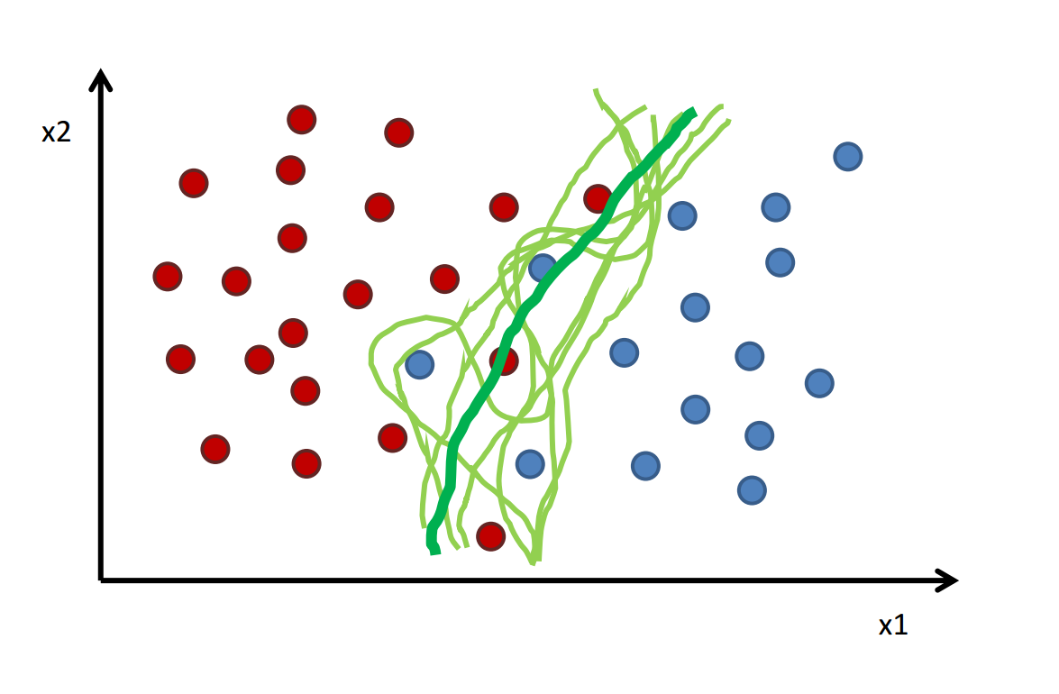
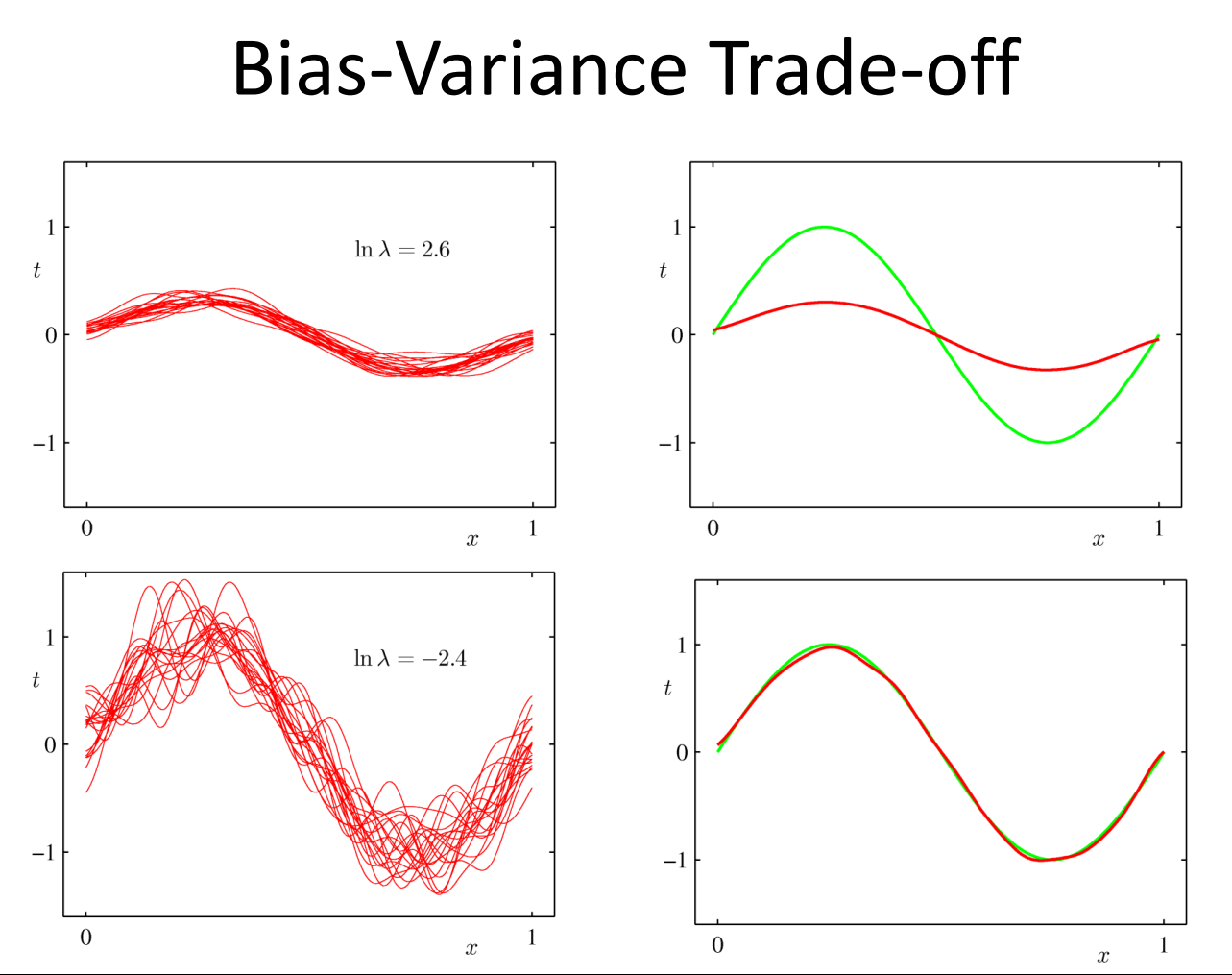
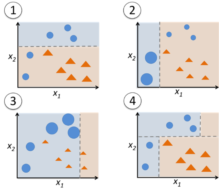
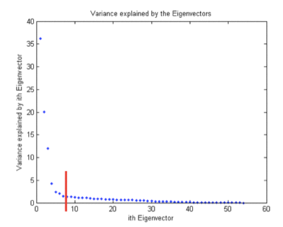
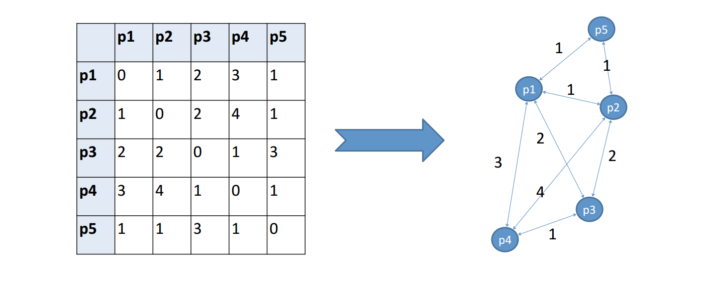
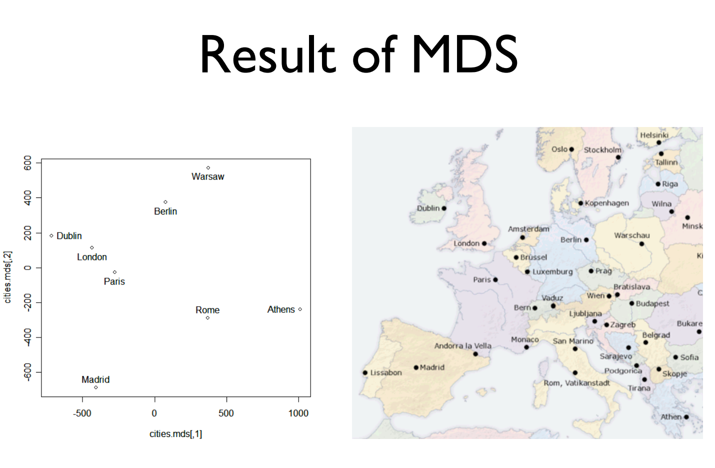
estimation risk
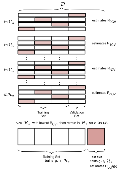
bootstrap
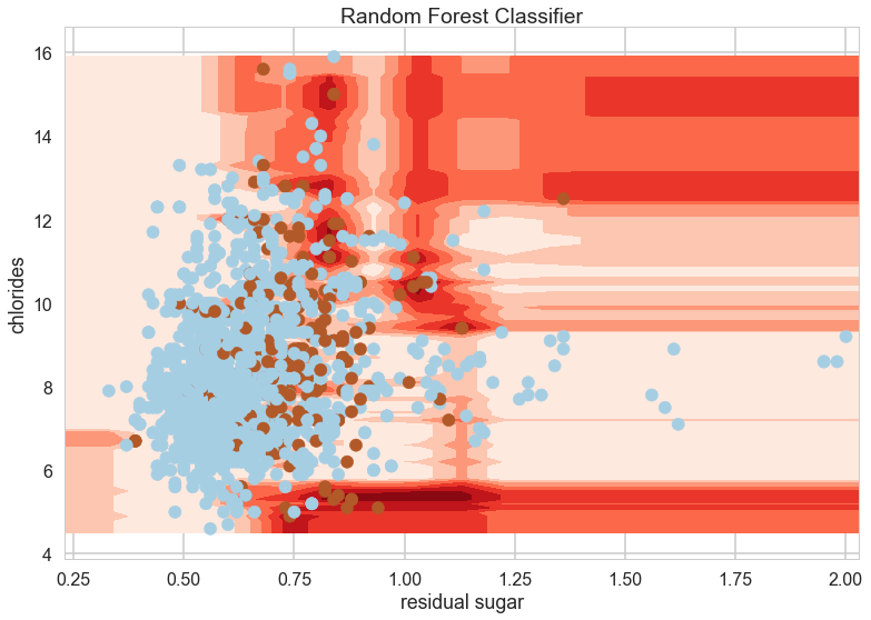
• Builds upon the idea of bagging
• Each tree build from bootstrap sample
• Node splits calculated from random feature subsets
• All trees are fully grown
• No pruning
• Two parameters
– Number of trees
– Number of features
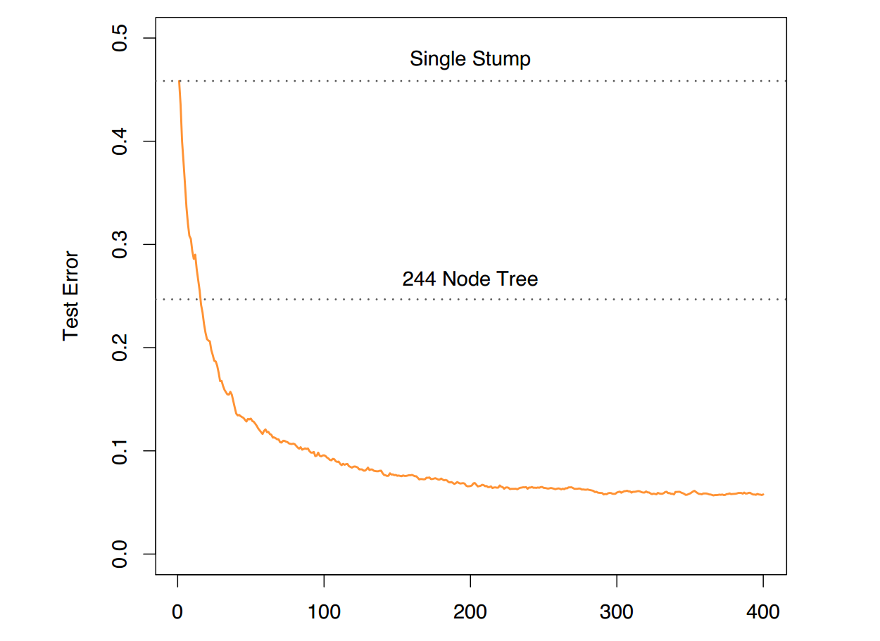
• Also ensemble method like Bagging
• But:
– weak learners evolve over time
– votes are weighted
• Better than Bagging for many applications
• number of trees
• number of splits in each tree (often stumps
work well)
• parameters controlling how weights evolve
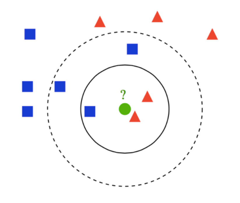
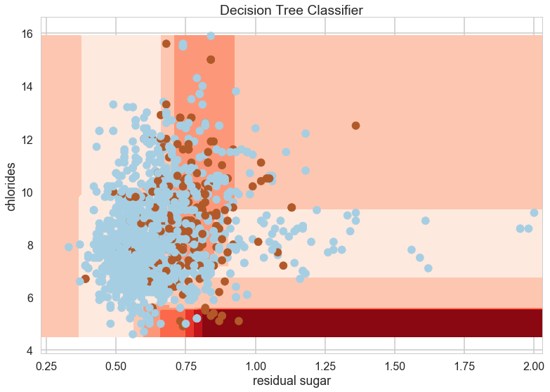
knn
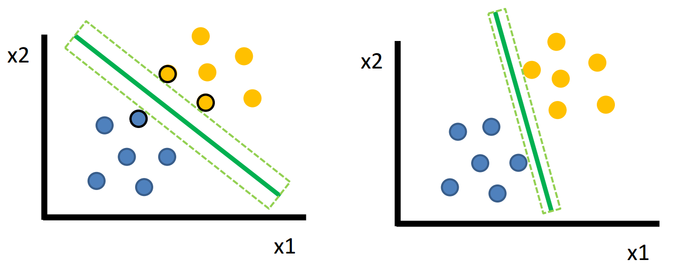
SVM
RF
deep learning
features
samples
1. Put a window around each point
2. Compute mean of points in the frame.
3. Shift the window to the mean
4. Repeat until convergence
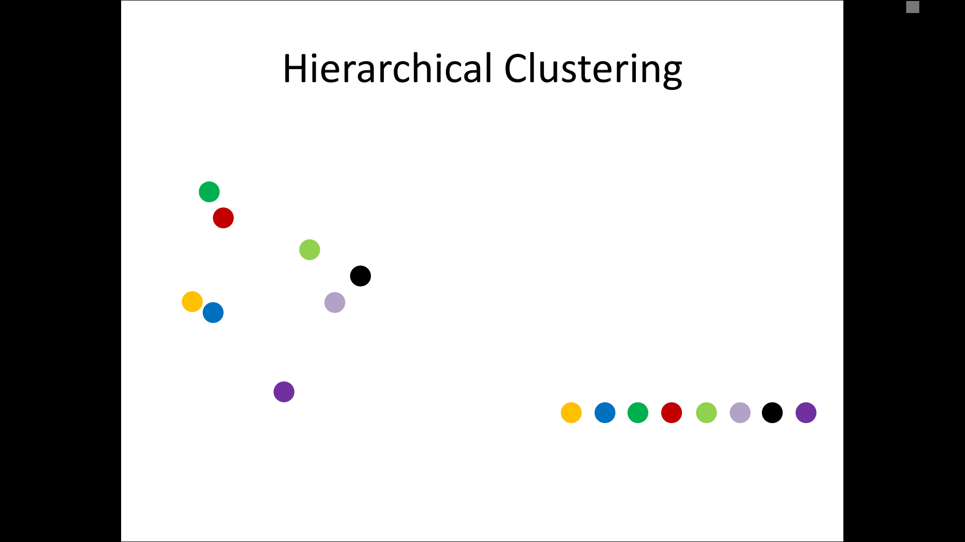
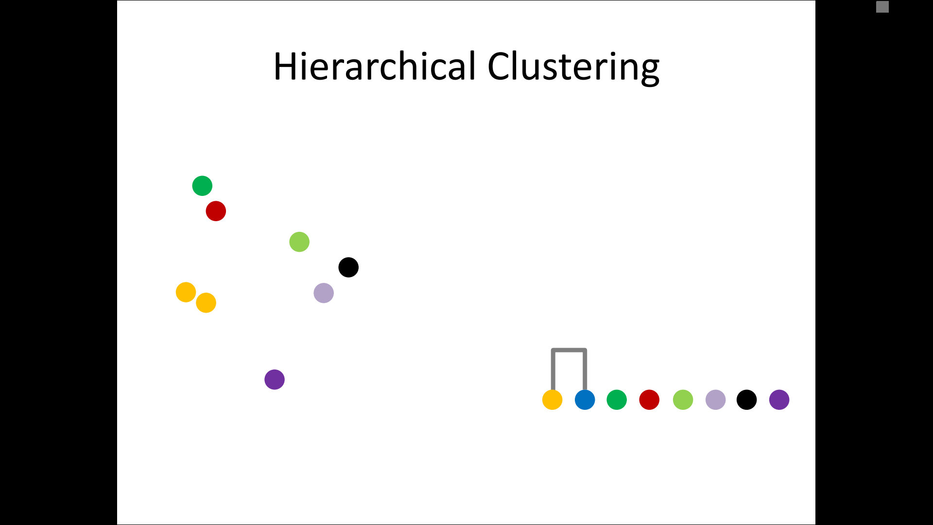
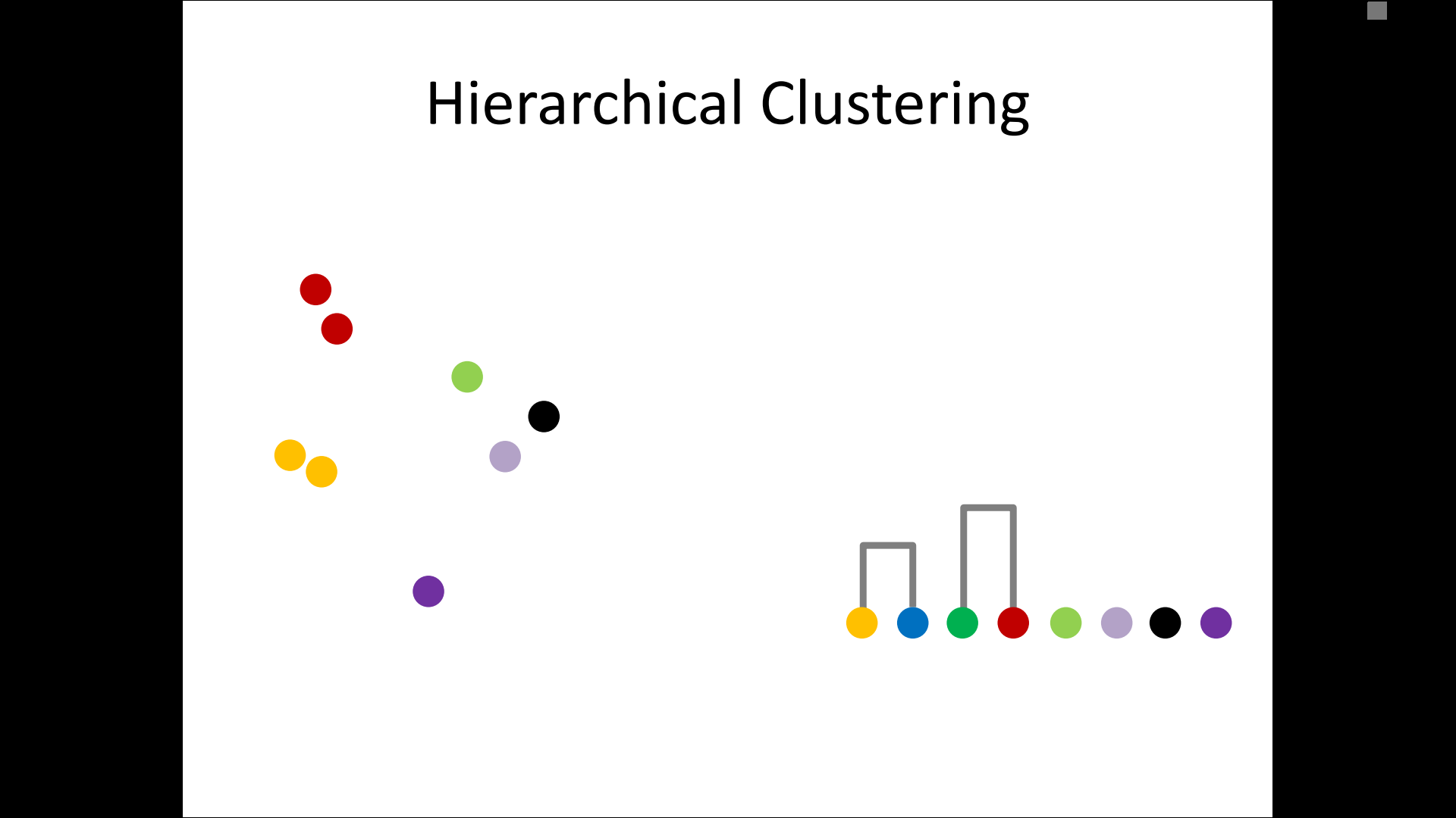
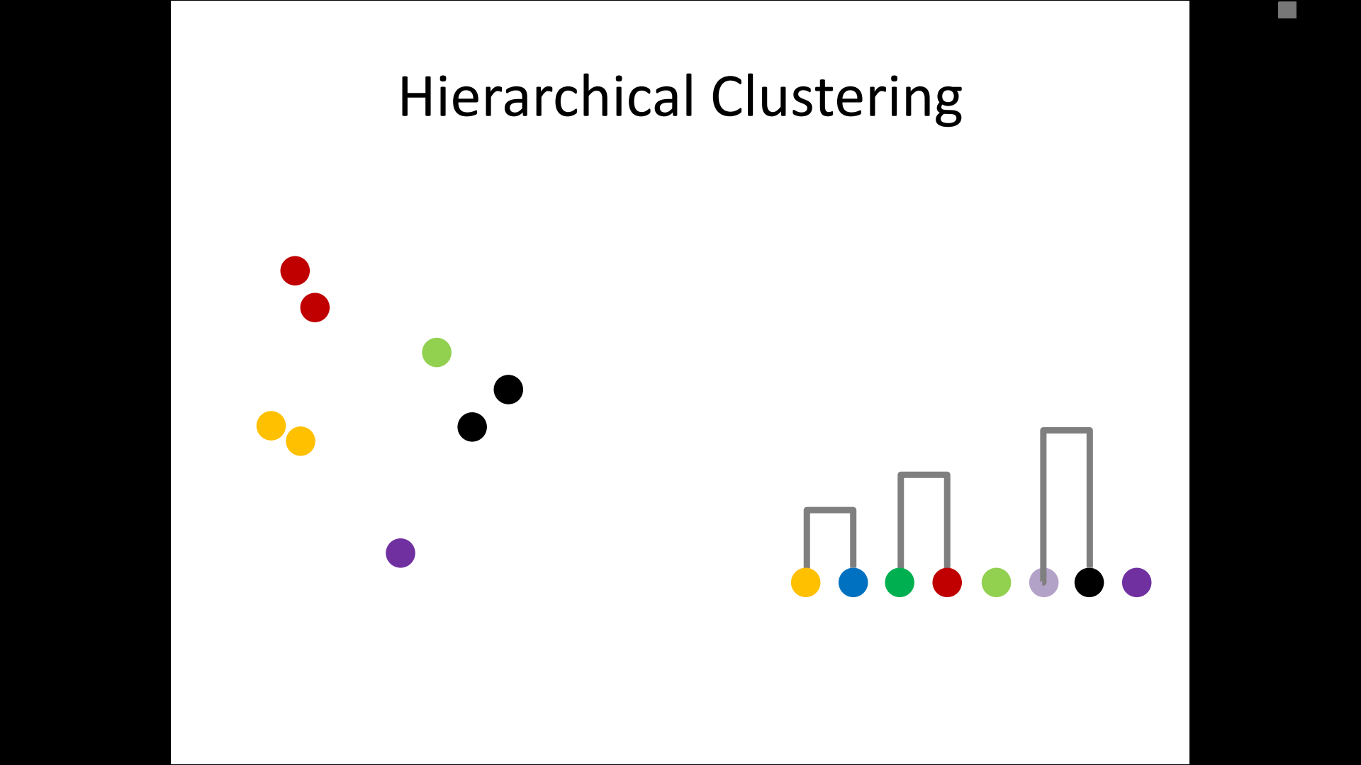
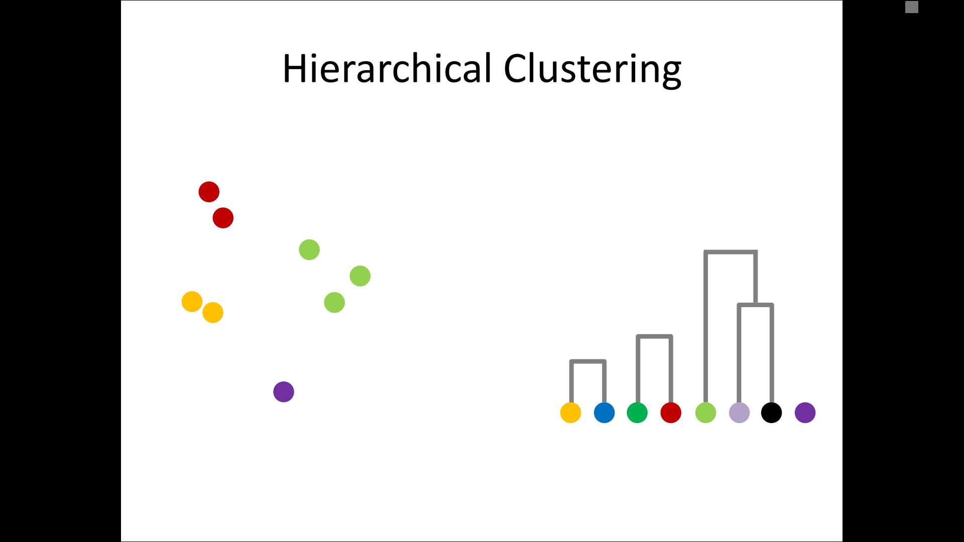
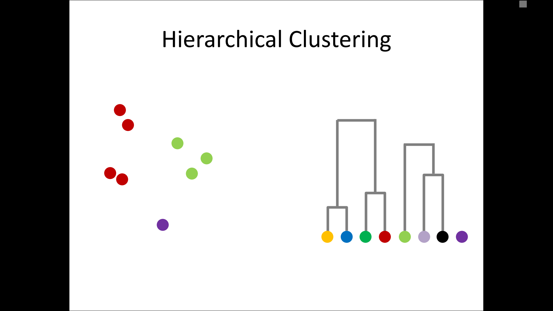
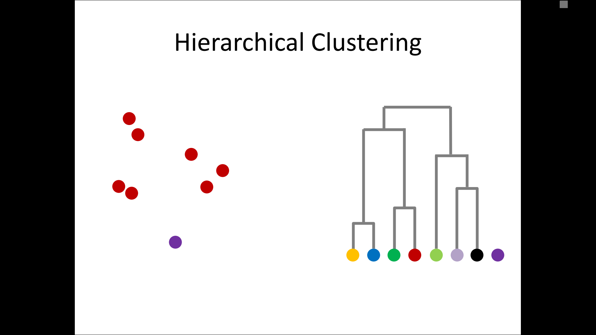
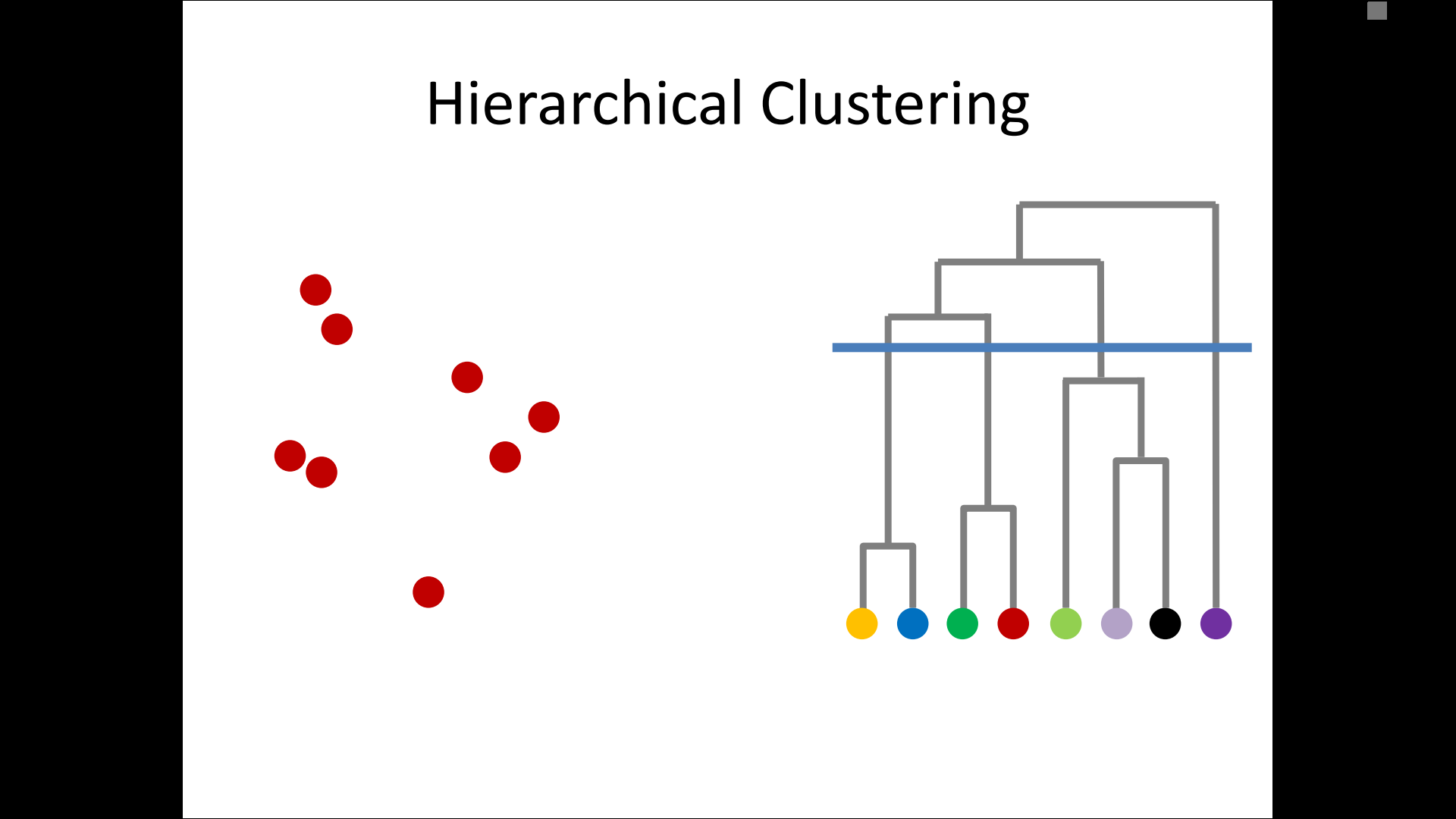
– single-linkage
– complete-linkage
– average linkage
decision risk
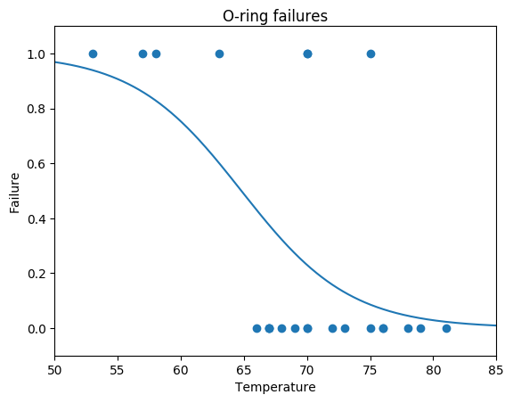
what else except accuracy/R^2 ?
Regression
MSE/MAE etc.
Classification
ROC P-R etc.
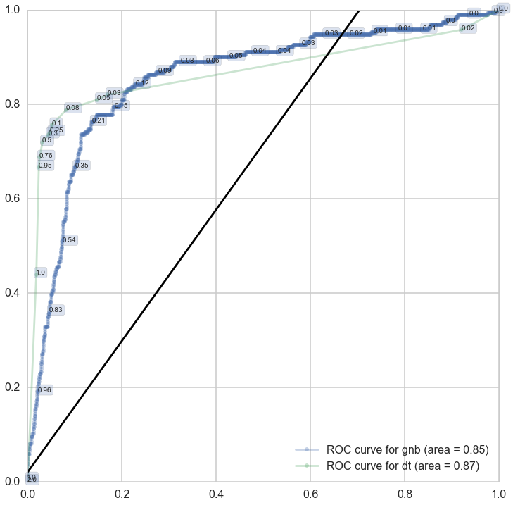
ROC
P-R
| predict fact |
1 |
0 |
|
|---|---|---|---|
| 1 | cost 1 | cost 2 | |
| 0 | cost 3 | cost 4 | |
cost matrix
終わり
By orashi


