

Patrick Power
Economics PhD @ Boston University
Patrick Power
The key facts of his career, which are that he knew (1) a lot about math and (2) nothing about finance. This seems to have been a very fruitful combination. If you can program computers to analyze data with, as it were, an open mind, they will pick out signals from the data that work, and then you can trade on those signals and make an enormous fortune. If you insist on the signals making sense to you, you will just get in the way.
Overview
In much of applied micro work, Causal Inference rests on the following condition
In many settings (Health Care, Education, Housing) we have the underlying text
(2) Illustrate that LLMs may particularly advantageous IV
Aim(s)
(1) Clarify the conditional independence assumption for text based controls
Motivation #-1
There are a lot of good reasons for not wanting to use LLMs for Causal Inference
Motivation #1 (Identification)
Motivation #2 (Efficiency)
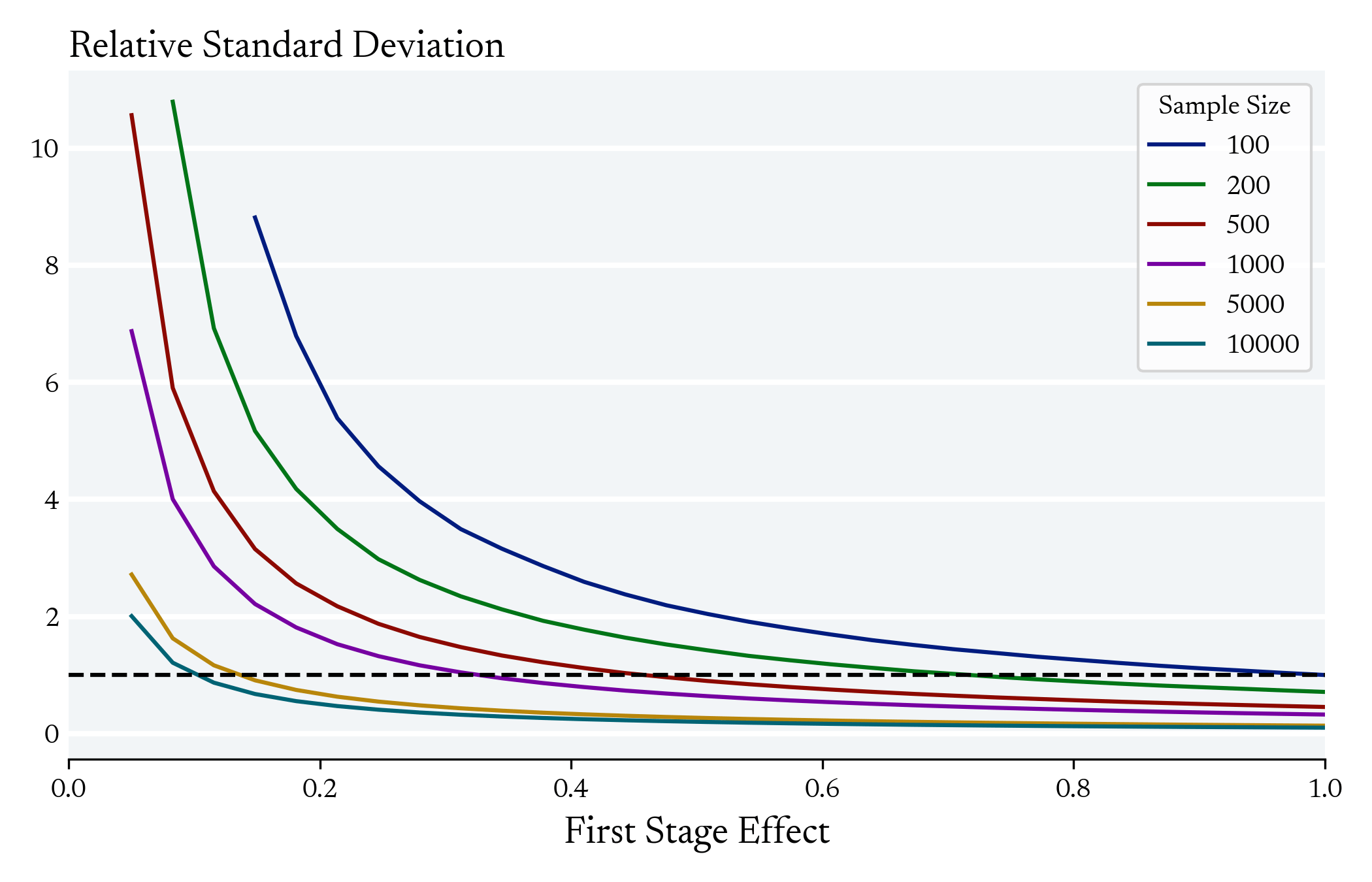
In instrumental variables, there can be an exponential relationship between the average first stage and the variance of the LATE estimator
Many Applied Microecon papers Exist in this range
But maybe there is "partial" information about who is a complier that language models can exploit in the first stage to reduce the variance
Motivation #2 (Efficiency)
Practitioners are often concerned about high take-up rates and therefore screen out individuals from the study
"We designed the consent and enrollment process for this RCT to yield high take-up rates, screening potential clients on their willingness to participate. In fact, about 91 percent of those in the treatment group who were offered services actually completed the initial assessment and received some services"
But you don't need to screen these individuals out before hand
Motivation #3 (Tranparency)
The Fundamental Challenge
The Product Topology Breaks Down
"You shall know a word by the company that it keeps" Firth [1957]
Words (Tokens)
The Real Numbers
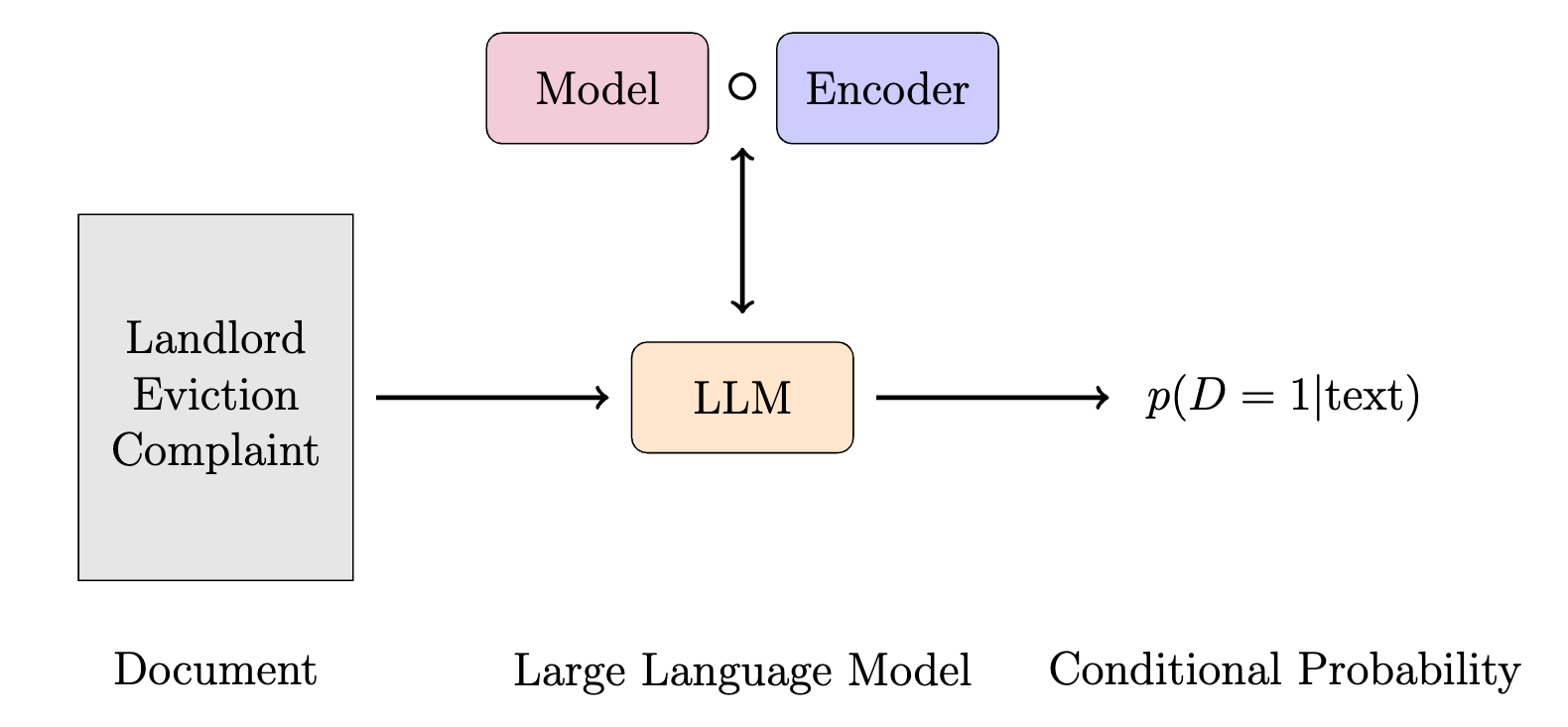
What Language Model Should We Use?
LLMs
Estimator
Project Data onto Low-Dimensional Manifold and Average locally
Maybe? But also latent
Estimator
Project Data onto Low-Dimensional Manifold and Average locally*
Probably Not Exactly True
Identification
Probably Not Exactly True
*Even linear models extrapolate
Causal Inference Doesn't Really Work
Conditional Expectation Function
When the treatment variable is conditional independent of the potential outcomes, the following holds
We approximate the Condition Expectation function via a parameterized model
In applied micro, the typical model is
Framework
In the standard Applied Micro Setup
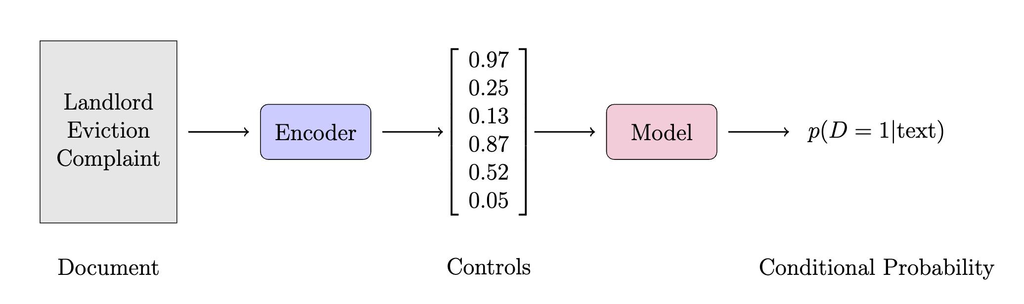
Encoder: Hand Selected Features
Model: Linear function of the control variables
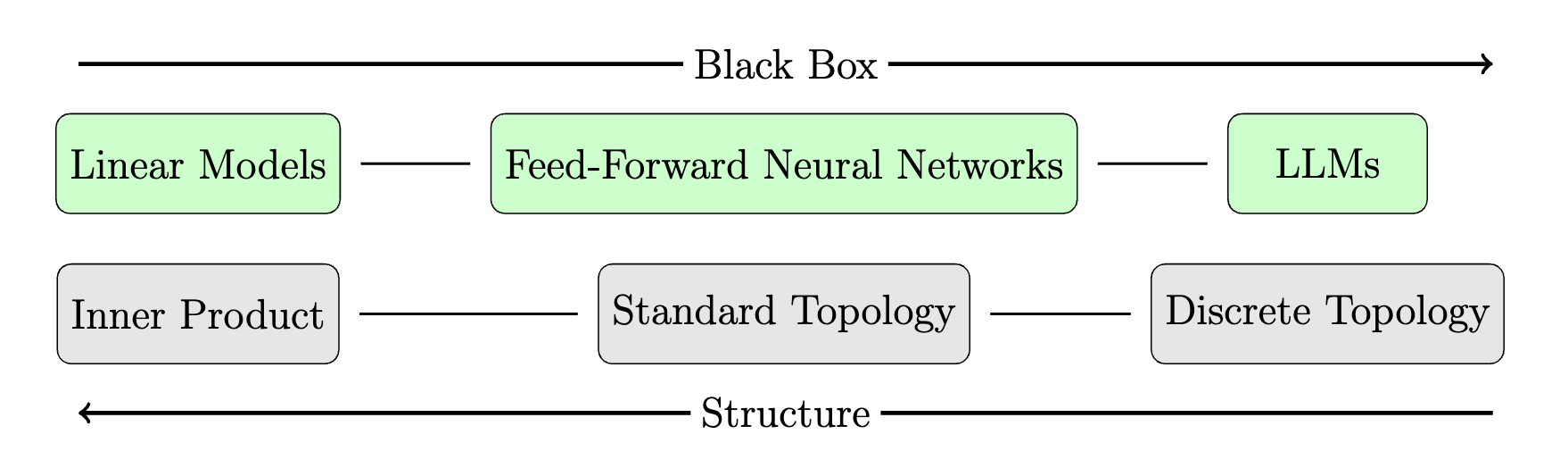
Topology provides necessary structure for Conditional Independence
The conditional expectation function defined with respect to the Borel sigma algebra generated with respect to the topology on X products out
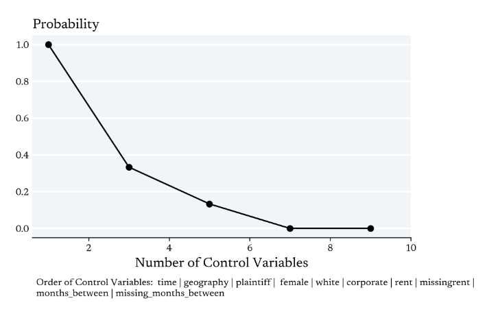
Adding Controls
More functions are continuous under the finer topology
Creates a "finer" topology on the underlying set
A finer topology places fewer restrictions on the Conditional Expectation Function
A finer topology also places fewer restrictions over our continuous model
A continuous function exploits meaningful variation
Unlike Homeomorphisms, continuous functions do not preserve all topological properties, but they do preserve the notion of "closeness"
Causal Framework
Conditional Independence
Model
Large Language Model
Causal Inference
We define the following random variables of interest
We begin with the underlying probability space
For notational simplicity, we take the treatment and outcome variables to be binary valued
Causal Inference
Conditional Independence
Identification
High Level Summary
Right to Counsel
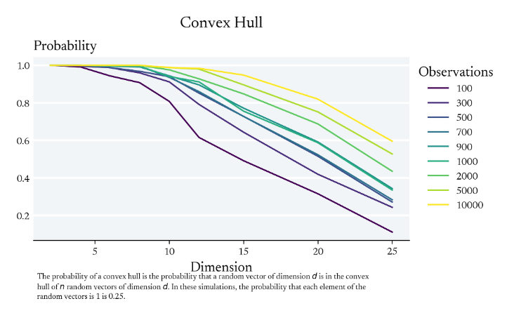
We're already Extrapolating with 'Vector' Data
Simulation
Motivation #2
What notion of similarity are we using to define Conditional Independence?
What notion of similarity are we using to form predictions from the training data?
Big Picture Overview
Undergraduate courses on Econometrics can be difficult to follow because they don't differentiate between these two notions of similarity
The Aim of this paper is to act as additional chapter of Mostly Harmless Econometrics focused on LLMs
The Mostly Harmless Econometric Approach is arguably more intuitive because it distinguishes between the two
Revisiting Controls
Language models can exploit features of the text which differentiate between these subpopulations and therefore "improve" estimation of IV parameters
Claim
(1) Doesn't change the first stage estimate
(2) Can decrease the variance of the LATE estimate
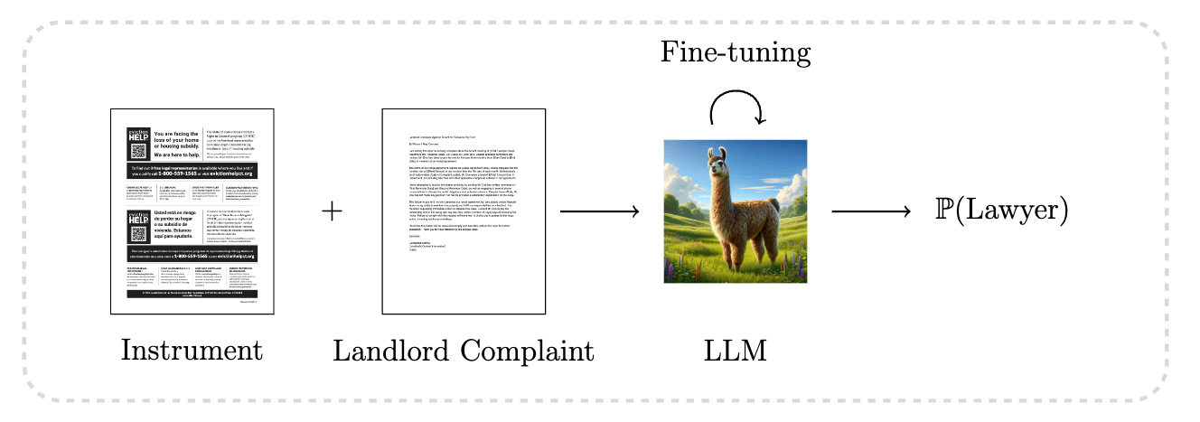
Motivational Example
Landlord Complaint
Examples
We observe aspects of the case which are potentially informative about who we receive legal representation if offered
Instrument Randomly Assigned
Models
Standard
Exploiting Heterogeneity
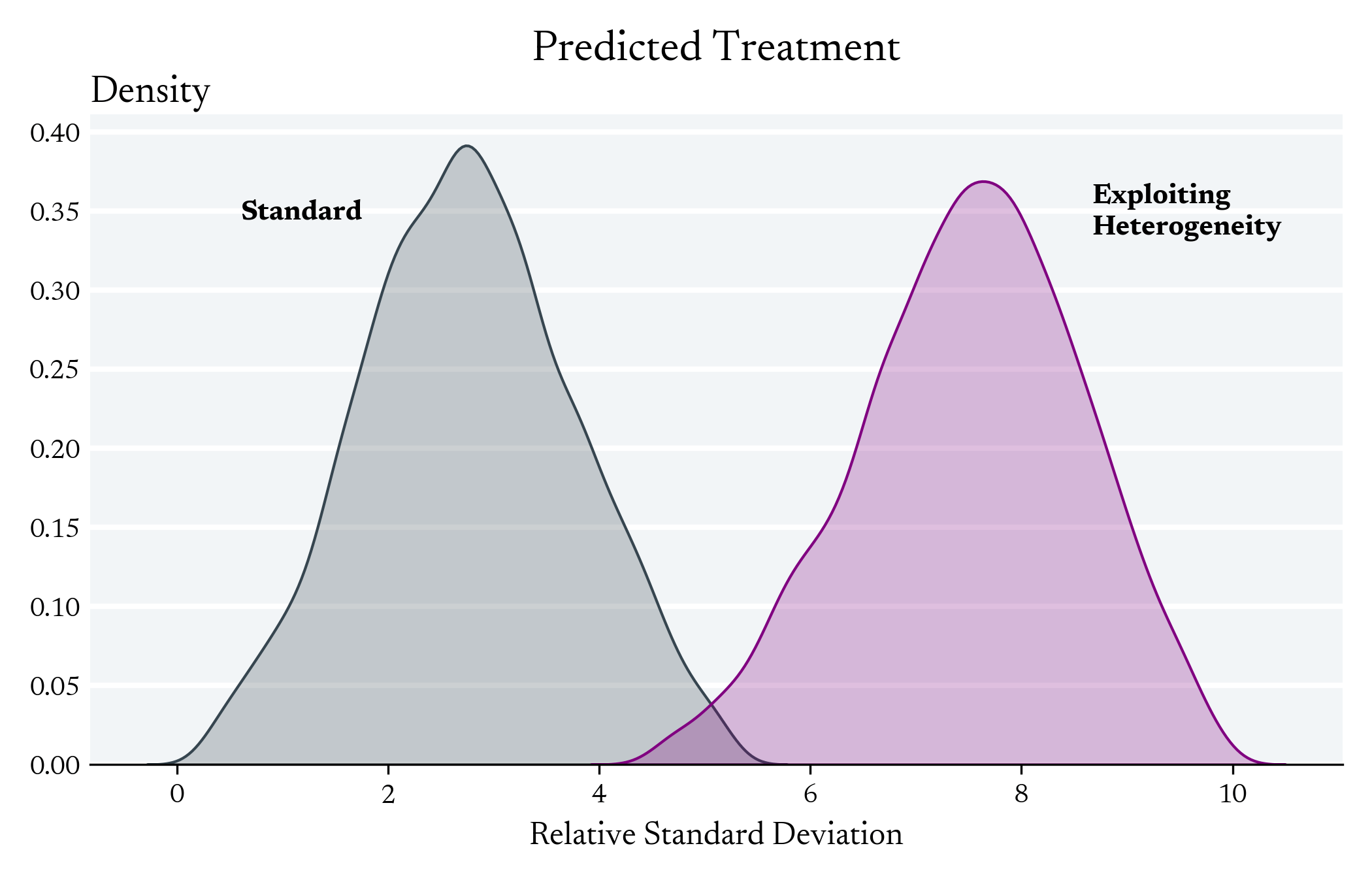
Exploiting Heterogeneity in the First Stage can Increase the Variance of Individual Level Predictions
First Stage Effect
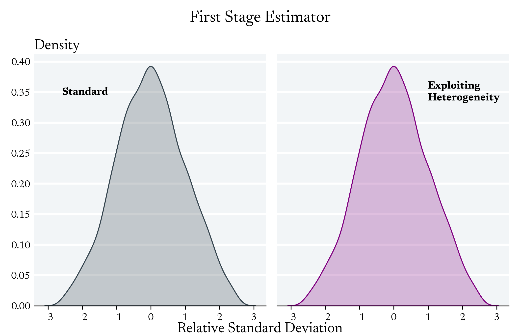
We don't expect to see differences between these models with regards to the Average First Stage Effect
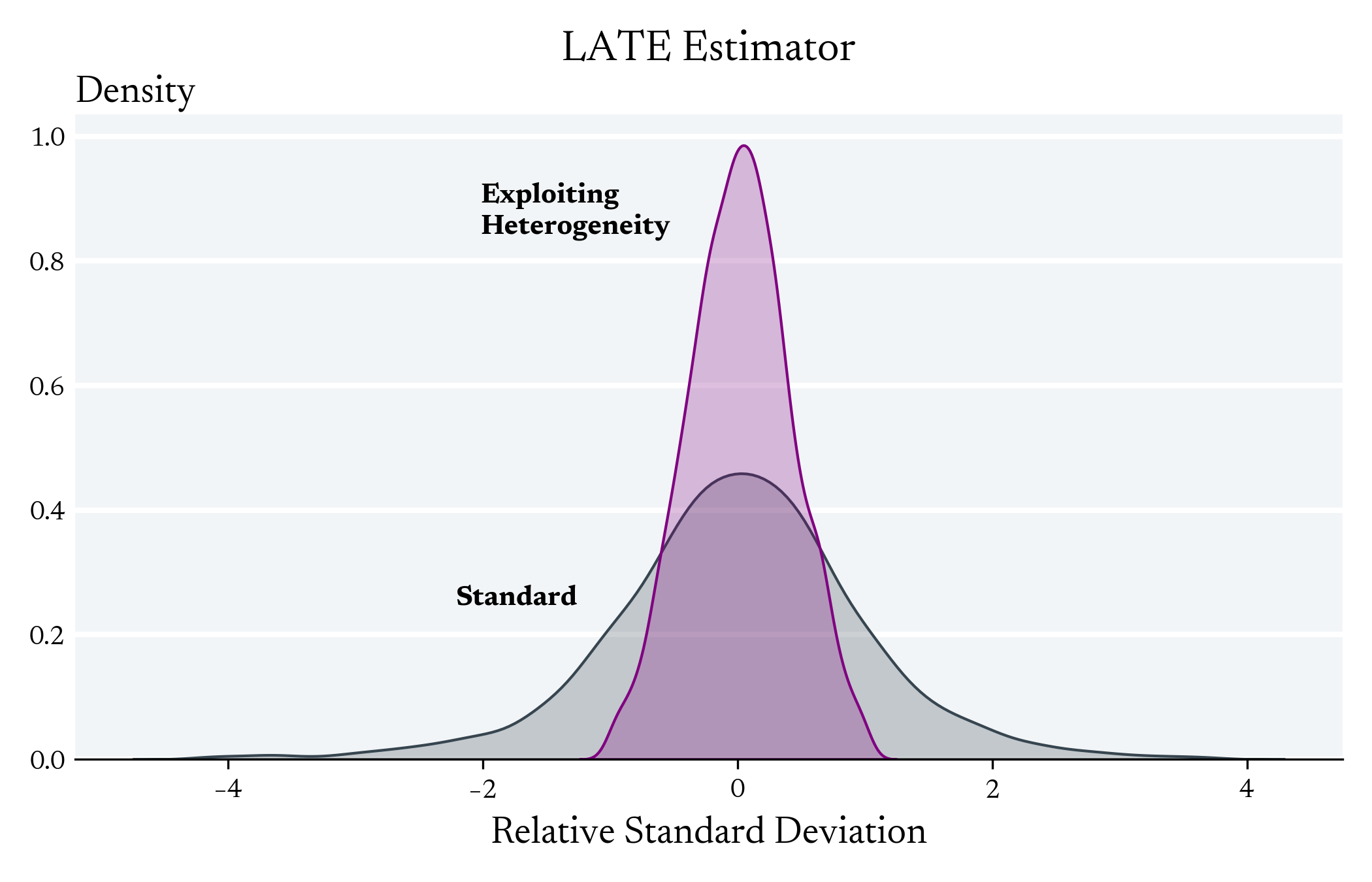
Exploiting Heterogeneity in the First Stage can Decrease the Variance the LATE Estimator
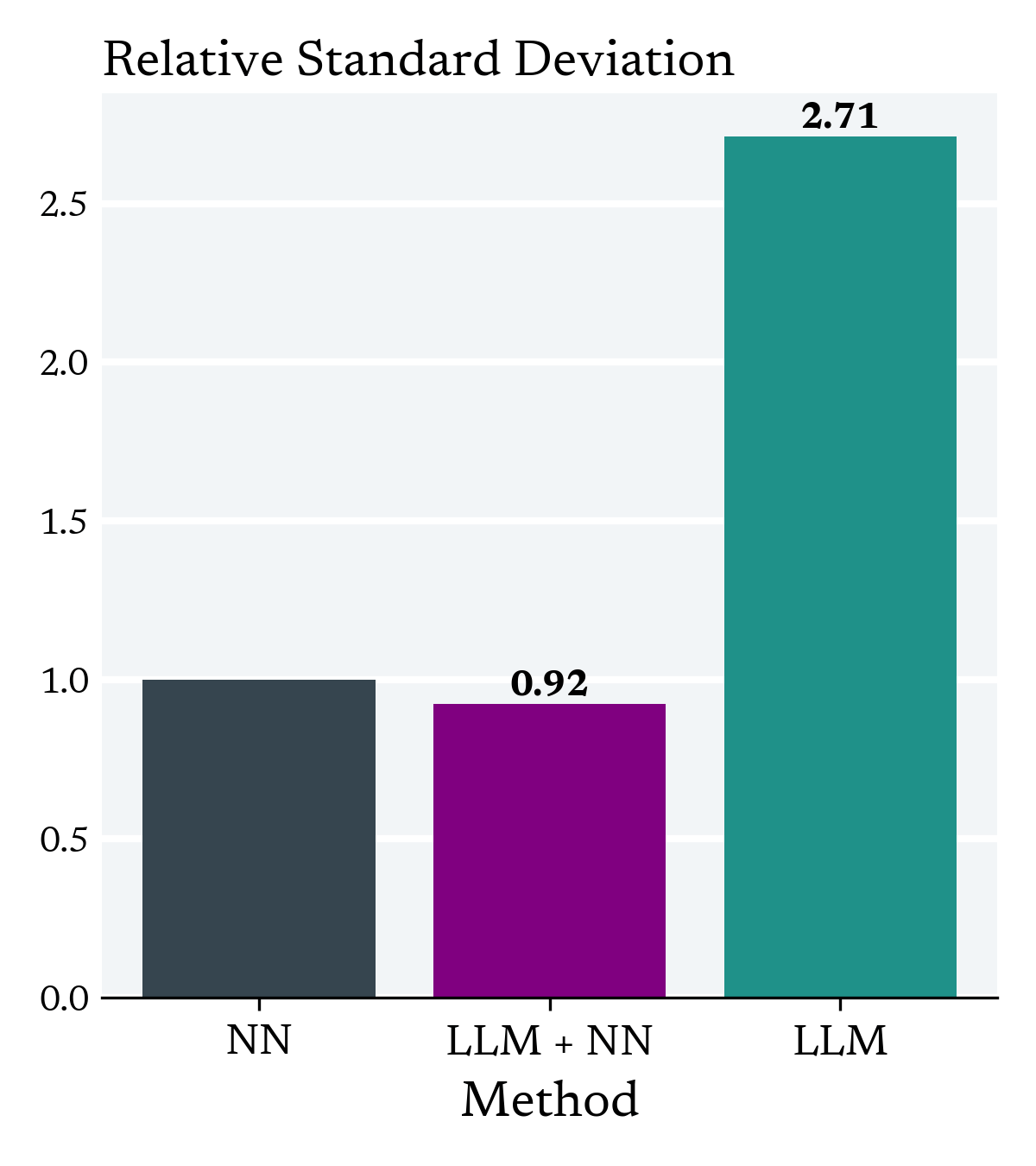
IV Simulation
(1)
Sample Numerical Features
(2)
Map Numerical Features to Text
via prompt
(3)
Define First Stage Function
(4)
(0)
Binary Instrument is Randomly Assigned
For computational reasons, we choose a simple first stage function so that we can learn it with relatively few observations
Context: Instrumental Variables with Preferential Treatment
Not clear how to make this work with a linear model
***For example, in Connecticut's rollout of the Right to Counsel, legal aid was offered in some zip codes initially but not others, and within these zip codes legal aid was prioritized to tenants who were more vulnerable
"The success of machine learning algorithms generally depends on data representation, and we hypothesize that this is because different representations can entangle and hide more or less the different explanatory factors of variation behind the data"
Representation Learning
"The performance of machine learning methods is heavily dependent on the choice of data representation (or features) on which they are applied. For that reason, much of the actual effort in deploying machine learning algorithms goes into the design of preprocessing pipelines and data transformations that result in a representation of the data that can support effective machine learning"
Selection-on-Observables
Partially Linear Models
The difference between treatment and the predicted treatment based only on the controls
Linear Models
Instrumental Variables
Linear IV
Partially Linear IV
By Patrick Power
In this paper, we assess the impact of the Right to Counsel in Eviction cases on housing stability.


