Approximate Bayesian Computation
& writing performant Python code
Patrick J. Laub and Pierre-Olivier Goffard
https://slides.com/plaub/abc & https://arxiv.org/abs/2007.03833

Background
- UQ Software engineering & math
- PhD (Aarhus & UQ): Computational applied probability
- Post-doc #1 (ISFA): Insurance applications
- Post-doc #2 (UoM): Empirical dynamic modelling

Motivation
Have a random number of claims \(N \sim p_N( \,\cdot\, ; \boldsymbol{\theta}_{\mathrm{freq}} )\) and the claim sizes \(U_1, \dots, U_N \overset{\mathrm{i.i.d.}}{\sim} f_U( \,\cdot\, ; \boldsymbol{\theta}_{\mathrm{sev}} )\).
We aggregate them somehow, like:
- aggregate claims: \(X = \sum_{i=1}^N U_i \)
- maximum claims: \(X = \max_{i=1}^N U_i \)
- stop-loss: \(X = ( \sum_{i=1}^N U_i - c )_+ \).
Question: Given a sample \(X_1, \dots, X_n\) of the summaries, what is the \(\boldsymbol{\theta} = (\boldsymbol{\theta}_{\mathrm{freq}}, \boldsymbol{\theta}_{\mathrm{sev}})\) which explains them?
Easier question: Given \((X_1, N_1), \dots, (X_n, N_n)\) summaries & counts, what is \(\boldsymbol{\theta}\)?
E.g. a reinsurance contract
Likelihoods
For simple rv's we know their likelihood (normal, exponential, gamma, etc.).
When simple rv's are combined, the resulting thing rarely has a likelihood.
$$ X_1, X_2 \overset{\mathrm{i.i.d.}}{\sim} f_X(\,\cdot\,) \Rightarrow X_1 + X_2 \sim ~ \texttt{Unknown Likelihood}! $$
For a sample of \(n\) i.i.d. observations the joint likelihood is
$$ p_{\boldsymbol{X}}(\boldsymbol{x} \mid \boldsymbol{\theta}) = \prod_{i=1}^n p_{X_i}(x_i; \boldsymbol{\theta}) \,. $$
If \(n\) increases, then \(p_{\boldsymbol{X}}(\boldsymbol{x} \mid \boldsymbol{\theta}) = \prod \text{Small things} \overset{\dagger}{=} 0\), or just takes a long time to compute, then \(\texttt{Intractable Likelihood}\)!
Usually it's still possible to simulate these things...
Bayesian statistics
Prior distribution \(\pi(\boldsymbol{\theta}) \)
Likelihood \(\pi( \boldsymbol{x} \mid \boldsymbol{\theta} )\)
Posterior distibution
$$ \pi(\boldsymbol{\theta} \mid \boldsymbol{x} ) = \frac{ \pi(\boldsymbol{\theta}) \pi( \boldsymbol{x} \mid \boldsymbol{\theta} ) }{ \pi( \boldsymbol{x} ) } $$

Markov chain Monte Carlo
Approximate Bayesian Computation
Example: Flip a coin a few times and get \((x_1, x_2, x_3) = (\text{H, T, H})\); what is
\pi(\theta | \boldsymbol{x}) ?
Exact matching algorithm
Given some observations \(\boldsymbol{x}_{\text{obs}}\), repeat:
- generate a potential parameter from the prior distribution \(\boldsymbol{\theta}^{\ast} \sim \pi(\boldsymbol{\theta})\);
- simulate some 'fake data' \(\boldsymbol{x}^{\ast}\) from the model \(\boldsymbol{\theta}^{\ast}\);
- if \( \boldsymbol{x}_{\text{obs}} = \boldsymbol{x}^{\ast}\), then store \(\boldsymbol{\theta}^{\ast}\).
The resulting \(\boldsymbol{\theta}^{\ast}\)s are an i.i.d. sample from the posterior \(\pi(\theta \mid \boldsymbol{x}_{\text{obs}})\).
Getting an exact match of the data is hard...
Accept fake data that's close to observed data
ABC acceptance–rejection algorithm
Given some observations \(\boldsymbol{x}_{\text{obs}}\), to generate \(R\) samples from the posterior:
- For \(i = 1\), \(\dots\), \(R\):
- Repeat:
- generate a potential parameter from the prior distribution \(\boldsymbol{\theta}^{\ast} \sim \pi(\boldsymbol{\theta})\);
- simulate some 'fake data' \(\boldsymbol{x}^{\ast}\) from the model \(\boldsymbol{\theta}^{\ast}\);
- Until \( \lVert \boldsymbol{x}_{\text{obs}}-\boldsymbol{x}^{\ast} \rVert \leq \epsilon\)
- Store \(\boldsymbol{\theta}^{\ast}_i = \boldsymbol{\theta}^{\ast}\)
- Repeat:
Inputs: \(\lVert \,\cdot\, \rVert\) denotes a distance measure, and \(\epsilon \ge 0\) is an acceptance threshold.
This samples from the approximate posterior a.k.a. the ABC posterior
$$ \pi_\epsilon(\boldsymbol{\theta} \mid \boldsymbol{x}_{\text{obs}}) \propto \pi(\theta) \times \mathbb{P}\bigl( \lVert \boldsymbol{x}_{\text{obs}}-\boldsymbol{x}^{\ast} \rVert \leq \epsilon \text{ where } \boldsymbol{x}^{\ast} \sim \boldsymbol{\theta} \bigr) . $$The 'approximate' part of ABC
ABC Sequential Monte Carlo
Main idea: Take a bad approximation and make a better one.
Say we have samples from a bad approximation \(\pi_3(\boldsymbol{\theta} \mid \boldsymbol{x}_{\text{obs}})\) and want to improve them to be samples from a better approximation \(\pi_1(\boldsymbol{\theta} \mid \boldsymbol{x}_{\text{obs}})\)?
- Fit a kernel density estimate \(K\) to the samples from the bad distribution \(\pi_3(\boldsymbol{\theta} \mid \boldsymbol{x}_{\text{obs}})\)
- For \(i = 1\), \(\dots\), \(R\):
- Repeat:
- generate a potential parameter \(\boldsymbol{\theta}^{\ast}\) from the KDE \(K\);
- simulate some 'fake data' \(\boldsymbol{x}^{\ast}\) from the model \(\boldsymbol{\theta}^{\ast}\);
- Until \( \lVert \boldsymbol{x}_{\text{obs}}-\boldsymbol{x}^{\ast} \rVert \leq 1\)
- Store \(\boldsymbol{\theta}^{\ast}_i = \boldsymbol{\theta}^{\ast}\) along with a weight \(w_i = \frac{ \pi(\boldsymbol{\theta}^{\ast}) }{ K(\boldsymbol{\theta}^{\ast}) }\)
- Repeat:
Repeat this to get the ABC Sequential Monte Carlo algorithm, a.k.a. Population Monte Carlo.
Dependent Poisson – Exponential variables

J. Garrido, C. Genest, and J. Schulz (2016), Generalized linear models for dependent frequency and severity of insurance claims, IME.
-
frequency \(N \sim \mathsf{Poisson}(\lambda=4)\),
-
severity \(U_i \mid N \sim \mathsf{DepExp}(\beta=2, \delta=0.2)\), defined as \( U_i \mid N \sim \mathsf{Exp}(\beta\times \mathrm{e}^{\delta N}), \)
-
summation summary \(X = \sum_{i=1}^N U_i \)
ABC posteriors based on 50 \(X\)'s and on 250 \(X\)'s given uniform priors.
ABC posterior vs true posterior
Observe \(X = \sum_{i=1}^N U_i\) where \(N \sim \mathsf{Poisson}(\lambda=4)\), \(U_i \mid N \sim \mathsf{DepExp}(\beta=2, \delta=0.2)\)
ABC posteriors (KDEs) based on 50 \(X\)'s and on 250 \(X\)'s.
True posteriors (histograms) based on all the \(N\)'s and \(U_i\)'s used to make the 50 \(X\)'s and the 250 \(X\)'s.


Code demonstration

Negative Binomial – Weibull variables
- frequency has negative binomial distribution \(N \sim \mathsf{NegBin}(\alpha=4, p=\frac23)\),
- severities have Weibull distributions \(U_i \sim \mathsf{Weibull}(k=\frac13, \beta=1)\),
- global stop-loss summary \(X = ( \sum_{i=1}^N U_i - 6 )_+\)
ABC posteriors based on 50 (11 non-zero) \(X\)'s and on 250 (69 non-zero) \(X\)'s with uniform priors.


Negative Binomial – Weibull variables: also observe the frequency
Observe \(X\) and \(N\) where \(X = ( \sum_{i=1}^N U_i - 6 )_+\), \(N \sim \mathsf{NegBin}(\alpha=4, p=\frac23)\) and \(U_i \sim \mathsf{Weibull}(k=\frac13, \beta=1)\).
ABC posteriors based on 50 (11 non-zero) \(X\)'s and on 250 (69 non-zero) \(X\)'s with uniform priors.


Same figure zoomed in...


Negative Binomial – Gamma variables (misspecified!)
- frequency has negative binomial distribution \(N \sim \mathsf{NegBin}(\alpha=4, p=\frac23)\),
- severities are fit with \(U_i \sim \mathsf{Gamma}(r, m)\) but generated by \(\mathsf{Weibull}(k=\frac13, \beta=1)\)
- global stop-loss summary \(X = ( \sum_{i=1}^N U_i - 6 )_+\)
ABC posteriors based on 50 (11 non-zero) \(X\)'s and on 250 (69 non-zero) \(X\)'s with uniform priors.


Model selection
Given some observations \(\boldsymbol{x}_{\text{obs}}\), to generate \(R\) samples from the posterior:
- For \(i = 1\), \(\dots\), \(R\):
- Repeat:
- choose a model \(m^{\ast} \sim \pi(m)\)
- generate a potential parameter from the prior distribution of that model \(\boldsymbol{\theta}^{\ast} \sim \pi(\boldsymbol{\theta} \mid m)\);
- simulate some 'fake data' \(\boldsymbol{x}^{\ast}\) from that parameter \(\boldsymbol{\theta}^{\ast}\);
- Until \( \lVert \boldsymbol{x}_{\text{obs}}-\boldsymbol{x}^{\ast} \rVert \leq \epsilon\)
- Store \(m^{\ast}_i = m^{\ast}\)
- Repeat:
Then the \(m^{\ast}\)s are samples from \(\pi(m \mid \boldsymbol{x}_{\text{obs}})\).
Model posterior: Weibull (✓) vs gamma (✗)?

ABC model posteriors based on 50 observations and on 250 observations.
ABC turns a statistics problem into a programming problem
... to be used as a last resort
Writing faster code
"Premature optimization is the root of all evil." Donald Knuth
Stop and ask why
\begin{aligned}
\text{Cost of computer's time saved}
&= \text{Computer \$/hr} \times \text{Fraction of wasteful code removed} \\
&\quad \times \text{Number of times the code is called} \times \text{Number of users}
\end{aligned}
\text{Cost of programmer's time spent optimizing}
\ll \text{Cost of computer's time saved}
A typical computer


A typical program
Time ->
Waiting to read or write data to memory

Source: Joel Fenwick's CSSE2310 lecture slides
Running


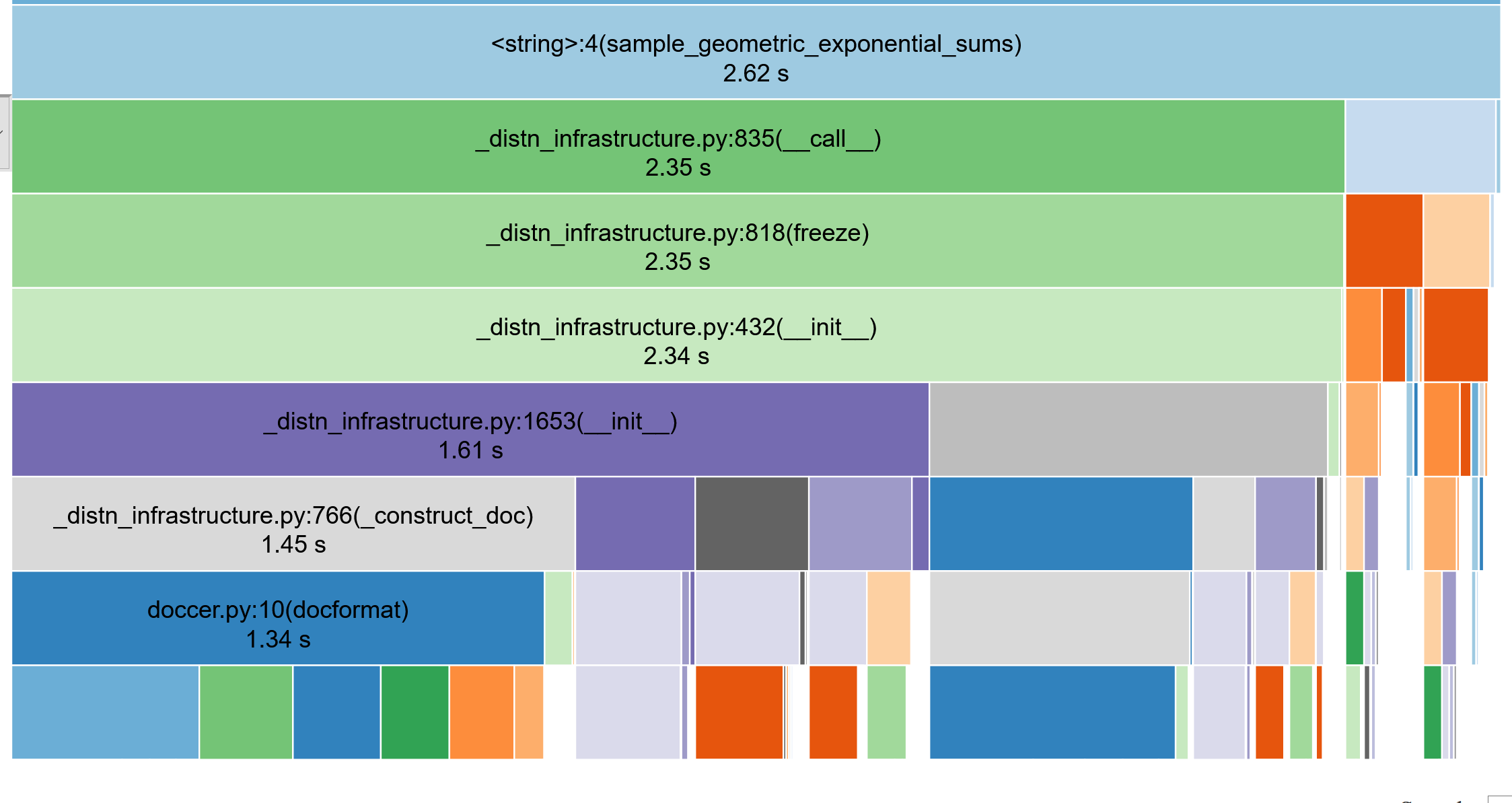
Profiling the code
(use snakeviz, lineprofiler)
from scipy import stats

def sample_geometric_exponential_sums(T, p, μ):
  result = []

  for t in range(T):
    N_t = stats.geom(p).rvs()
    X_t = 0.0
    for n in range(N_t):
      U_n = stats.expon(μ).rvs()
      X_t += U_n

    result.append(X_t)

  return result
Typically need to call this \(10^7\) times
\mathbf{X} = (X_t)_{t = 1, \dots, T}
X_t = \sum_{n=1}^{N_t} U_n
N_t = stats.geom(p).rvs()N_t = stats.geom.rvs(p)1.7 s vs 89 ms ... (19x speedup)

import numpy.random as rnd

def sample_geometric_exponential_sums(T, p, μ):
  result = []

  for t in range(T):
    N = rnd.geometric(p)

    X_t = 0.0
    for n in range(N):
      U_n = rnd.exponential(μ)
      X_t += U_n

    result.append(X_t)

  return result
Looking in the source, see that scipy just wraps numpy
Down from 89 ms to 5.5 ms (another 16x speedup)
Vectorised code
(use numpy)
Benefits of vectorised code
- Readability; more concise, expressing high-level ideas, e.g.
- Replace slow interpreted loops with fast compiled code
- Potentially can use a CPU's vectorised instructions (SIMD)
- Better use of the CPU's cache
\[ \sum_{n=0}^{\infty} \frac{f^{(n)}(a)}{n!} (x-a)^n \]
def sample_geometric_exponential_sums(T, p, μ):
  result = []

  for t in range(T):
    N = rnd.geometric(p)

    X_t = 0.0
    for n in range(N):
      X_t += rnd.exponential(μ)

    result.append(X_t)

  return result
Unvectorised
def sample_geometric_exponential_sums(T, p, μ):
  X = np.zeros(T)
  N = rnd.geometric(p, size=T)

  for t in range(T):
    X[t] = rnd.exponential(μ, size=N[t]).sum()

  return X
Vectorised (& most readable)
5.5 ms to 5.48 ms (no change)
def sample_geometric_exponential_sums(T, p, μ):
  X = np.zeros(T)

  N = rnd.geometric(p, size=T)
  U = rnd.exponential(μ, size=N.sum())

  i = 0
  for t in range(T):
    X[t] = U[i:i+N[t]].sum()
    i += N[t]

  return X
5.5 ms to 2.7 ms (2x speedup)
Allocate all random variables in one hit
Compiled code
(use numba)

C.f. Lin Clark (2017), A crash course in JIT compilers
https://hacks.mozilla.org/2017/02/a-crash-course-in-just-in-time-jit-compilers/
Talking to a computer
Interpreters & compilers
C.f. Lin Clark (2017), A crash course in JIT compilers


What does a machine understand?
Intel i5 (2010): add (0101), subtract (1111), ...
Intel i7 (2020): add (0101), subtract (1111), add_vectors (1011), ...
Apple M1 (2020): add (100), subtract (111), ...
\underbrace{\text{1100 0111}}_{\Large \text{function}}~\underbrace{\text{0100 0101 1111 1000 0000}}_{\Large \text{arg1}}~\underbrace{\text{0001 0000 0000 0000 0000 0000 0000}}_{\Large \text{arg2}}
movl $0x1, -0x8(%rbp)int x = 1;Instruction set architecture (ISA), e.g. x86-64
Try Compiler Explorer https://godbolt.org/z/dTv78M
Why is Python slow?
x = 1
y = 2
z = x + y

x = "Patrick "
y = "Laub"
z = x + y
int x = 1;
int y = 2;
int z = x + y;
std::string x2 = "Patrick ";
std::string y2 = "Laub";
std::string z2 = x2 + y2;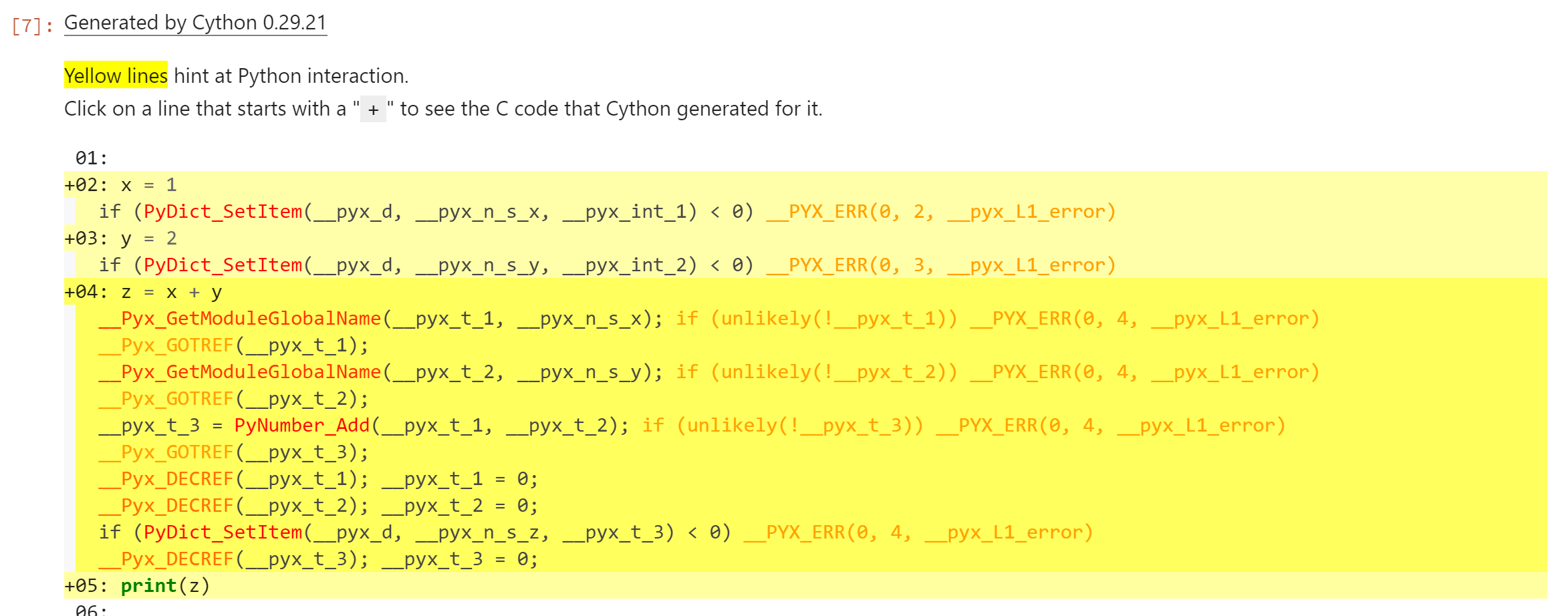
Try Compiler Explorer https://godbolt.org/z/dTv78M
// x = 1
if (PyDict_SetItem(__pyx_d, __pyx_n_s_x, __pyx_int_1) < 0) {
__PYX_ERR(0, 2, __pyx_L1_error);
}

// y = 2
if (PyDict_SetItem(__pyx_d, __pyx_n_s_y, __pyx_int_2) < 0) {
__PYX_ERR(0, 3, __pyx_L1_error);
}

// z = x + y
__Pyx_GetModuleGlobalName(__pyx_t_1, __pyx_n_s_x);
if (unlikely(!__pyx_t_1)) {
__PYX_ERR(0, 4, __pyx_L1_error);
}
__Pyx_GOTREF(__pyx_t_1);
__Pyx_GetModuleGlobalName(__pyx_t_2, __pyx_n_s_y);
if (unlikely(!__pyx_t_2)) {
__PYX_ERR(0, 4, __pyx_L1_error);
}
__Pyx_GOTREF(__pyx_t_2);
__pyx_t_3 = PyNumber_Add(__pyx_t_1, __pyx_t_2);
if (unlikely(!__pyx_t_3)) {
__PYX_ERR(0, 4, __pyx_L1_error);
}
__Pyx_GOTREF(__pyx_t_3);
__Pyx_DECREF(__pyx_t_1);
__pyx_t_1 = 0;
__Pyx_DECREF(__pyx_t_2);
__pyx_t_2 = 0;
if (PyDict_SetItem(__pyx_d, __pyx_n_s_z, __pyx_t_3) < 0) {
__PYX_ERR(0, 4, __pyx_L1_error);
}
__Pyx_DECREF(__pyx_t_3);
__pyx_t_3 = 0;
Python
C++
def arraySum(arr):
  sum = 0;
  for i in range(len(arr)):
    sum += arr[i];

  return sum
C.f. Lin Clark (2017), A crash course in JIT compilers
https://hacks.mozilla.org/2017/02/a-crash-course-in-just-in-time-jit-compilers/
def sample_geometric_exponential_sums(T, p, μ):
  X = np.zeros(T)

  N = rnd.geometric(p, size=T)
  U = rnd.exponential(μ, size=N.sum())

  i = 0
  for t in range(T):
    X[t] = U[i:i+N[t]].sum()
    i += N[t]

  return X
Interpreted version
cpdef sample_geometric_exponential_sums(long T, double p, double mu):
  cdef double[:] X = np.zeros(T)
  cdef long[:] N = rnd.geometric(p, size=T)
  cdef double[:] U = rnd.exponential(mu, size=np.sum(N))

  cdef int i = 0
  cdef int t
  for t in range(T):
    X[t] = np.sum(U[i:i+N[t]])
    i += N[t]
    return X
Compiled by Cython (not recommended)
def sample_geometric_exponential_sums(T, p, μ):
  X = np.zeros(T)

  N = rnd.geometric(p, size=T)
  U = rnd.exponential(μ, size=N.sum())

  i = 0
  for t in range(T):
    X[t] = U[i:i+N[t]].sum()
    i += N[t]

  return X
Interpreted version
from numba import njit

@njit()
def sample_geometric_exponential_sums(T, p, μ):
  X = np.zeros(T)

  N = rnd.geometric(p, size=T)
  U = rnd.exponential(μ, size=N.sum())

  i = 0
  for t in range(T):
    X[t] = U[i:i+N[t]].sum()
    i += N[t]

  return X
First run is compiling (500 ms), but after we are
down from 2.7 ms to 164 μs (16x speedup)
Compiled by numba
Original code: 1.7 s
Basic profiling with snakeviz: 5.5 ms, 310x speedup
+ Vectorisation/preallocation with numpy: 2.7 ms, 630x speedup
+ Compilation with numba: 164 μs, 10,000x speedup
And potentially:
+ Parallel over 80 cores: say another 50x improvement,
so overall 50,000x speedup.
Parallel code
(use joblib)
Computing in parallel
serialResult = sum(f(i) for i in range(n+1))

from joblib import Parallel, delayed

with Parallel(n_jobs=10) as parallel:
  parResult = sum(parallel(delayed(f)(i) for i in range(n+1)))
In python, use joblib. E.g. to calculate
\[ \sum_{i=0}^{n} f(i) \]
Multiple threads or multiple processes?
Use multiple processes in Python,
probably should use multiple threads elsewhere.

Baumann et al. (2019), A fork() in the road
17th Workshop on Hot Topics in Operating Systems


Amdahl’s Law (or Law of Diminishing Returns)
\(P\) is the proportion of a program that can be made parallel
\( 1 - P \) remains serial.
Theoretical maximum speedup of achieved by N processor is
\[ S(N)=1/[(1-P)+P/N] \]
Hence with unlimited processor count
\[ S(\infty) = 1 / (1-P) \]
E.g. \(P = 0.9\) then \( S(\infty) = 10 \).
Theoretical limits
In practice..
Either:
- too much parallelism for the computer
- a problem which is too small for the parallelism
Know your CPU

Intel lies
Apple confuses

>>> import psutil

>>> psutil.cpu_count()
4

>>> psutil.cpu_count(logical=False)
2
Apple is cooler (literally)
# This tells Python to just use one thread for internal
# math operations. When it tries to be smart and do multithreading
# it usually just stuffs everything up and slows us down.
import os
for env in ["MKL_NUM_THREADS", "NUMEXPR_NUM_THREADS", "OMP_NUM_THREADS"]:
    os.environ[env] = "1"
sample_abc_population(N)
sample_one()
sample_one()
sample_one()
sample_one()
np.solve(A, x)
parfor i = 1:m
  for j = 1:n
    f(i, j)
  end
end
for i = 1:m
parfor j = 1:n
f(i, j)
end
end

11.9 s
41.8 s
class Parallel(Logger):

  """

  ...

  batch_size: int or 'auto', default: 'auto'
            The number of atomic tasks to dispatch at once to each
            worker. When individual evaluations are very fast, dispatching
            calls to workers can be slower than sequential computation because
            of the overhead. Batching fast computations together can mitigate
            this.
            The ``'auto'`` strategy keeps track of the time it takes for a batch
            to complete, and dynamically adjusts the batch size to keep the time
            on the order of half a second, using a heuristic. The initial batch
            size is 1.
            ``batch_size="auto"`` with ``backend="threading"`` will dispatch
            batches of a single task at a time as the threading backend has
            very little overhead and using larger batch size has not proved to
            bring any gain in that case.

    ...


    """
https://github.com/joblib/joblib/blob/master/joblib/parallel.py
Contributions
- Modest theoretical contribution, looking at convergence of the approximate posterior to the true posterior in the case of mixed data (e.g. truncated data).
- An optimized parallel Python package abcre ('re' for reinsurance), on Github
Take-home messages
- What ABC can do, when to use it (as a last resort)
- ABC turns a statistics problem into a programming problem
- Profile your code (snakeviz)
- Vectorise your code (numpy)
- Compile your code (numba)
- Parallelise your code (joblib), don't overdo it
ABC talk (UNSW)
By plaub


