Rare-event asymptotics and estimation for dependent random sums


Exit Talk of Patrick J. Laub

University of Queensland & Aarhus University

PhD outline

2015 Aarhus
2016 Jan-Jul Brisbane
2016 Aug-Dec Aarhus
2017 Brisbane/Melbourne
2018 Jan-Apr (end) China

   Supervisors: Søren Asmussen, Phil Pollett, and Jens L. Jensen
\sum ~ \infty

10101

Sums of random variables

Asymptotic analysis / rare-events

Monte Carlo simulation

What is applied probability?

Data

Fitted model

Decision

Statistics

App. Prob.

You have some goal..

Insurance
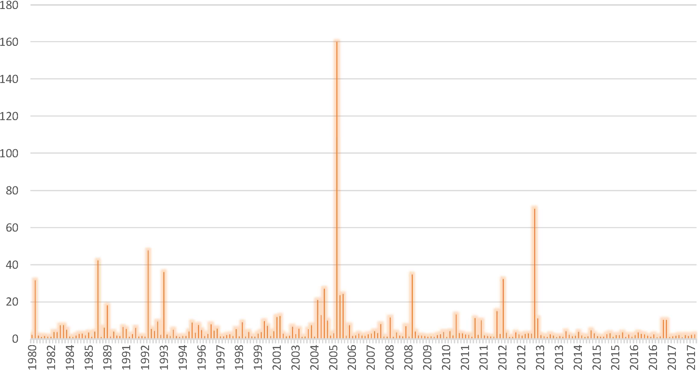
Estimated financial cost of the natural disasters in the USA which cost over $1bn USD. Source: National Centers for Environmental Information
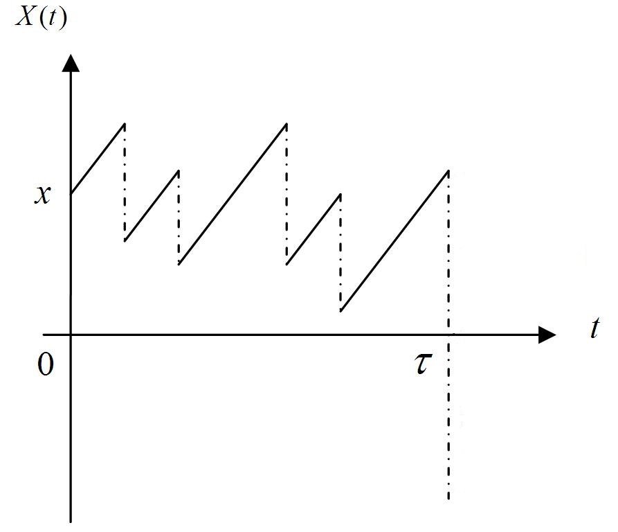
Cramér-Lundberg model

Interested in

  • Probability of ruin (bankruptcy) in the next 10 years 
  • Probability of ruin eventually
  • Stop-loss premiums
\mathbb{E}[ (X - a)_+ ] = \mathbb{E}[ \min\{ X-a, 0 \} ]

E.g. guaranteed benefits

\text{Death benefits} = \text{Value of stock portfolio}
\text{or if too small, some guaranteed threshold}

An investor's problems

\text{Portfolio} = \text{IBM} + \text{Google} + \text{Facebook} + \ldots
\mathbb{P}(\text{Portfolio} < x)

Want to know:

  - cdf values


  - value at risk


  - expected shortfall

\text{VaR}_{1\%} = \text{ With 99\% probability I'll lose less than this amount}
\text{ES}_{1\%} = \text{ How much I expect to lose in the 1\% worst-case scenario}

Modelling stock prices

Black, F., & Scholes, M. (1973). The pricing of options and corporate liabilities. Journal of political economy

Fischer Black            Myron Scholes

Can you tell which is BS?
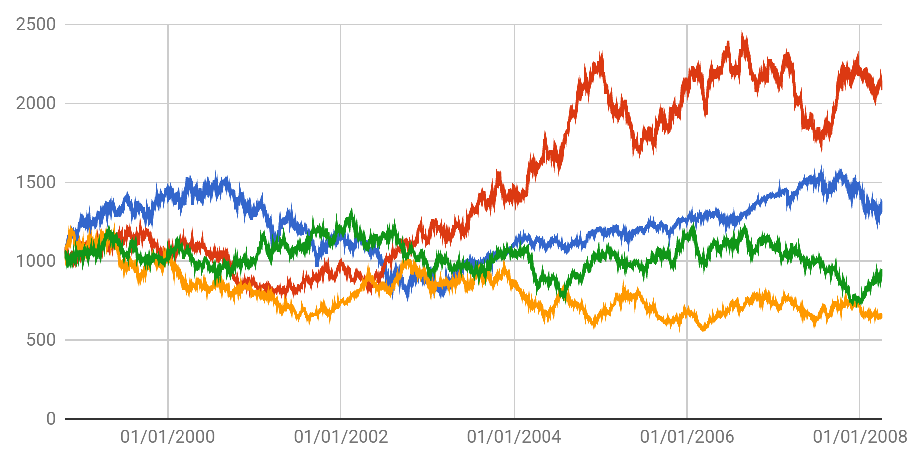
S&P 500 from Oct 1998 to Apr 2008

Google Finance

Geometric Brownian motion

\frac{\mathrm{d}S_t}{S_t} = \mu \, \mathrm{d}t + \sigma \, \mathrm{d}W_t
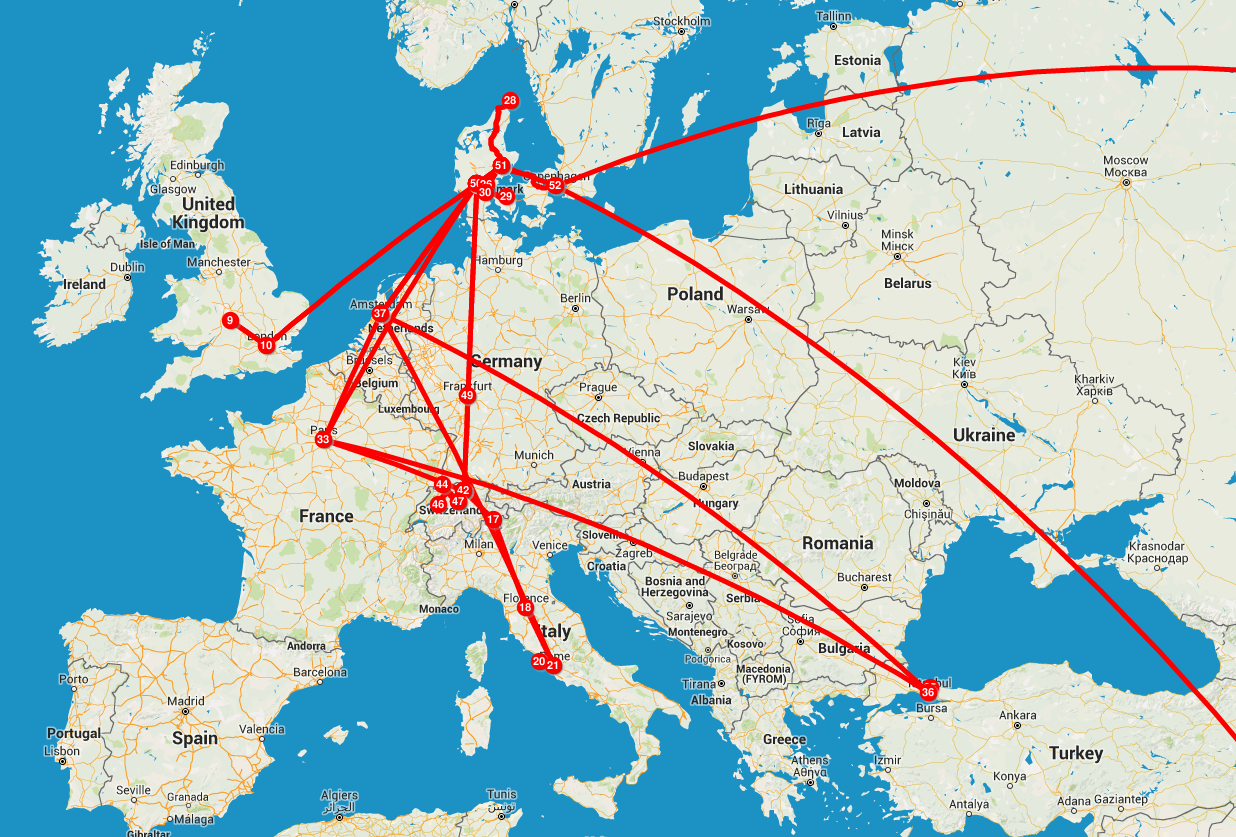
\Rightarrow S_t \sim \mathsf{Lognormal}

In words, Stock Price = (Long-term) Trend + (Short-term) Noise

That's just the beginning..

General diffusion processes...

\mathrm{d}S_t = \mu_t(S_t) \mathrm{d}t + \sigma(S_t) V_t \, \mathrm{d}W_t + \kappa(S_t) \mathrm{d} N_t

Stochastic volatility processes...

\mathrm{d}S_t = \mu_t(S_t) \mathrm{d}t + \sigma(S_t) \mathrm{d}W_t

SV with jumps...

\mathrm{d}S_t = \mu_t(S_t) \mathrm{d}t + \sigma(S_t) V_t \, \mathrm{d}W_t

SV with jumps governed by a Hawkes process with etc...

Monte Carlo

\mathbb{P}(\text{Hitting the dartboard}) = \frac{\text{Area(dartboard)}}{\text{Area(square)}}
= \frac{\pi r^2}{(2 r)^2} = \frac{\pi}{4}
\mathbb{P}(\text{Hitting the dartboard}) \approx \frac{\text{\# hits of board}}{\text{\# throws}}
\Rightarrow \pi \approx 4 \times \frac{\text{\# hits of board}}{\text{\# throws}}

Quasi-Monte Carlo

For free, you get a confidence interval

Sum of lognormals distributions

S = X_1 + X_2 + \ldots + X_d
X \sim \mathsf{Lognormal}(\mu, \Sigma)

where

S \sim \mathsf{SumLognormal}(\mu, \Sigma)

What is that?

Start with a multivariate normal
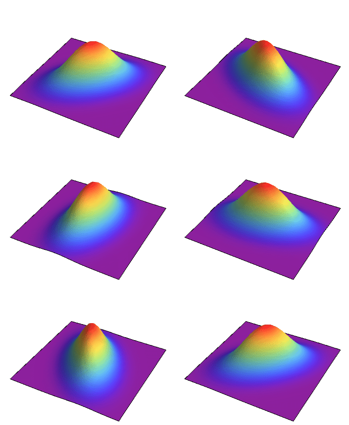
X = \exp\{Z\}
Z \sim \mathsf{Normal}(\mu, \Sigma)

Then set 

Then add them up

What's known about sums?

S = X_1 + \ldots + X_d
\mathbb{E}[S] = \sum_{i=1}^n \mathbb{E}[X_i]
\mathscr{L}_S(t) \equiv \mathbb{E}[ \mathrm{e}^{-t S} ] = \mathscr{L}_{X_1}(t) \times \ldots \times \mathscr{L}_{X_d}(t)
f_{S}(s) = \left(f_{X_1} * \ldots * f_{X_n}\right)(s) = \int_{1 \cdot x = s} f_{X}(x) \mathrm{d} x

Easy to calculate interesting things with the density

Density can be known..

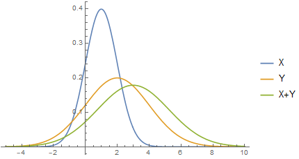
X \sim \mathsf{Normal}(\mu_1,\sigma_1^2), Y \sim \mathsf{Normal}(\mu_2, \sigma_2^2) \Rightarrow X+Y \sim \mathsf{Normal}(\mu_1+\mu_2, \sigma_1^2 + \sigma_2^2)

Example

X \sim \mathsf{Gamma}(r_1, m), Y \sim \mathsf{Gamma}(r_2, m) \Rightarrow X+Y \sim \mathsf{Gamma}(r_1+r_2, m)
X \sim \mathsf{Lognormal}(\mu_1, \sigma_1^2), Y \sim \mathsf{Lognormal}(\mu_2, \sigma_2^2) \Rightarrow X+Y \sim \mathsf{Lognormal}(\ldots, \ldots)

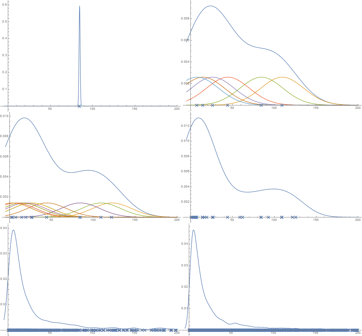
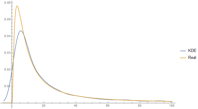
Kernel-density estimation

Laplace transform approximation

\mathscr{L}_X(t) = \overline{\mathscr{L}}_X(t) (1 + \mathcal{O}(\frac{1}{\log(t)}))

No closed-form exists for a single lognormal

Asmussen, S., Jensen, J. L., & Rojas-Nandayapa, L. (2016). On the Laplace transform of the lognormal distribution. Methodology and Computing in Applied Probability

Generalise to d dimensions

  1. Setup Laplace's method
  2. Find the maximiser
  3. Apply Laplace's method
\mathscr{L}_S(t) \text{ for } S \sim \mathsf{SumLognormal}(\mu, \Sigma)

Laub, P. J., Asmussen, S., Jensen, J. L., & Rojas-Nandayapa, L. (2016). Approximating the Laplace transform of the sum of dependent lognormals. Advances in Applied Probability

Generalise to d dimensions

  1. Setup Laplace's method
  2. Find the maximiser
  3. Apply Laplace's method
= \frac{ \exp\left\{ (1 - \frac12 x^* )^\top \Sigma^{-1} x^* \right\} }{\sqrt{\det(\Sigma H)}} (1 + \mathcal{o}(1))
\mathscr{L}_S(t) = \mathbb{E}( \mathrm{e}^{-t S} ) = \mathbb{E}( \mathrm{e}^{-t (\mathrm{e}^{X_1} + \ldots + \mathrm{e}^{X_d}) } )
= \frac{1}{\sqrt{(2\pi)^d \det(\Sigma)}} \int_{\mathbb{R}^d} \exp \{ {-}t \, 1^\top \mathrm{e}^{\mu + x} -\frac12 x^\top \Sigma^{-1} x \} \mathrm{d} x
{-}t \mathrm{e}^{\mu + x^*} = \Sigma^{-1} x^*

Solve numerically: 

\mathscr{L}_S(t) = \overline{\mathscr{L}}_S(t) (1 + \mathcal{o}(1))
H = t \, \mathrm{diag}( \mathrm{e}^{\mu + x^*} ) + \Sigma^{-1}

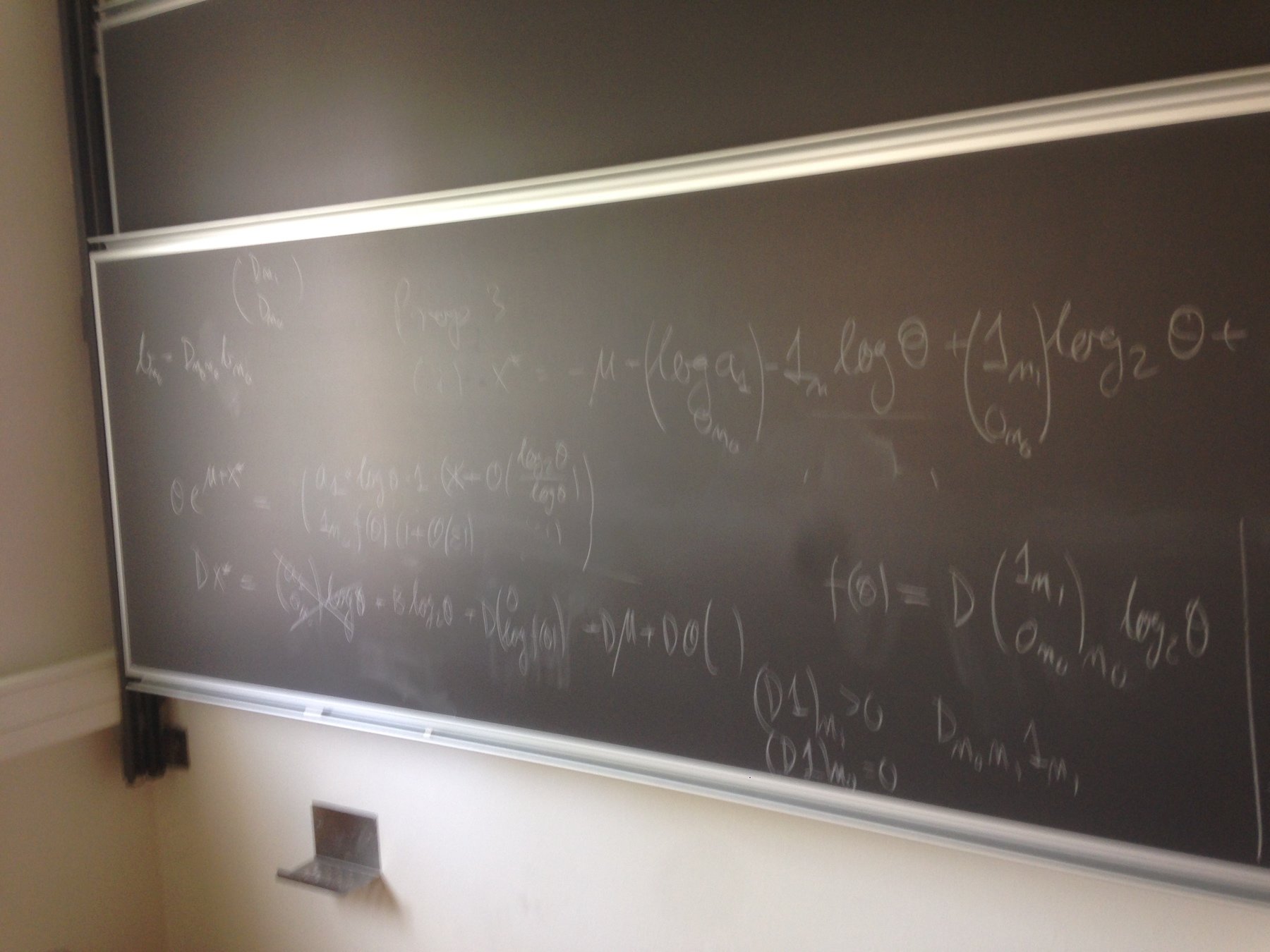
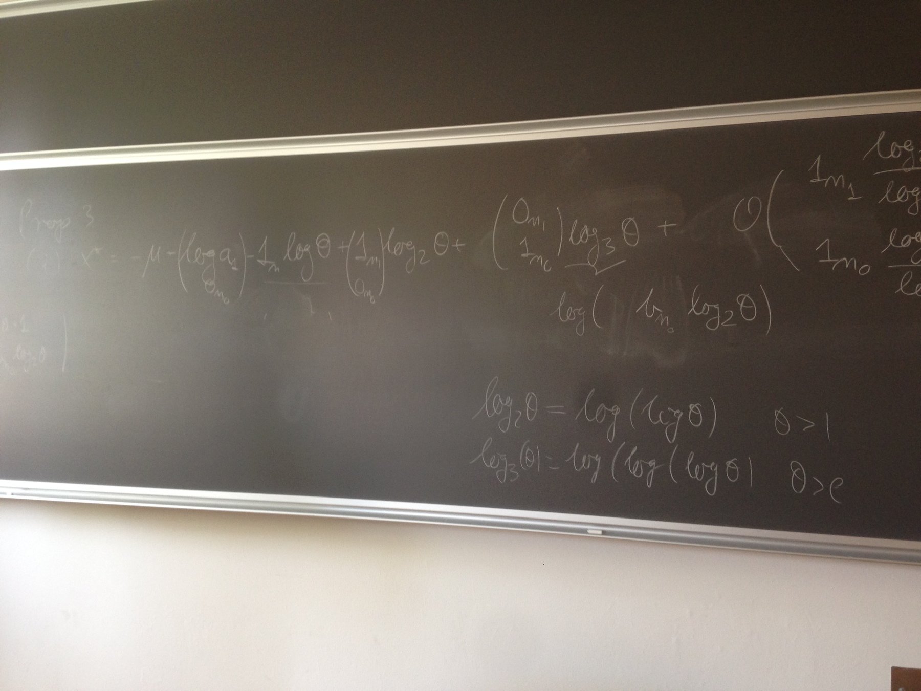
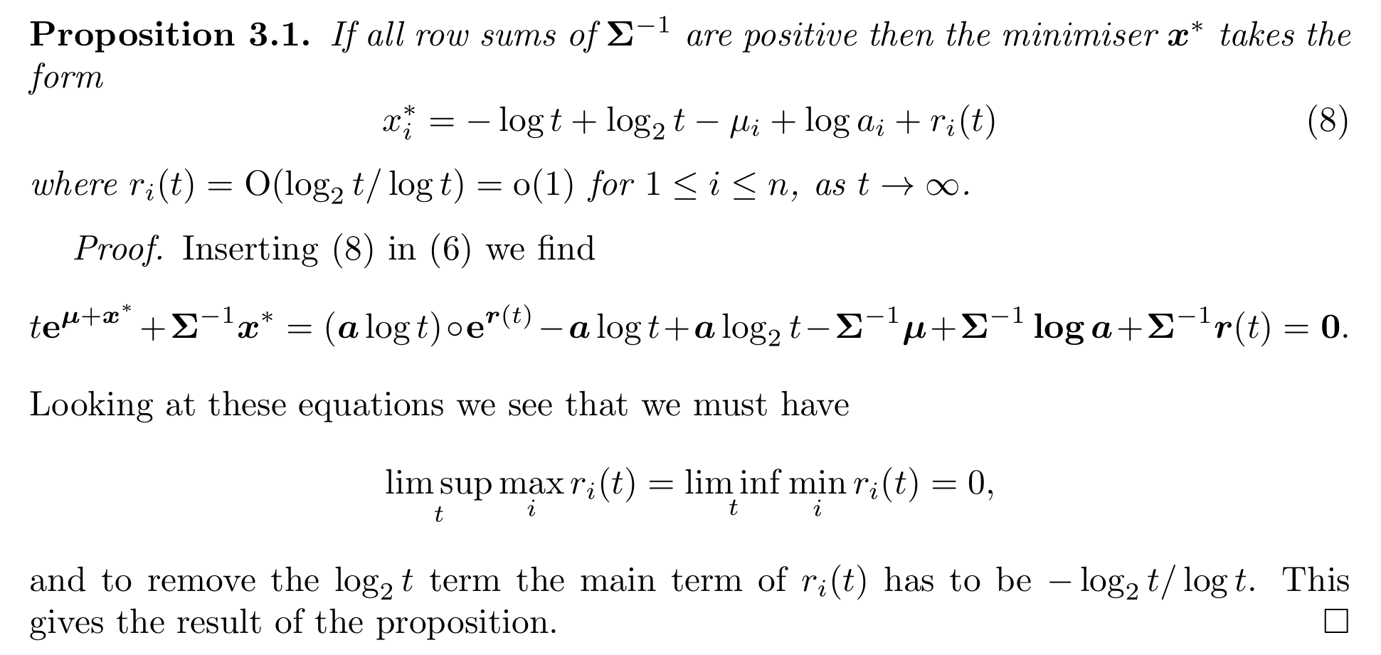
What is the maximiser?

{-}t \mathrm{e}^{\mu + x^*} = \Sigma^{-1} x^*
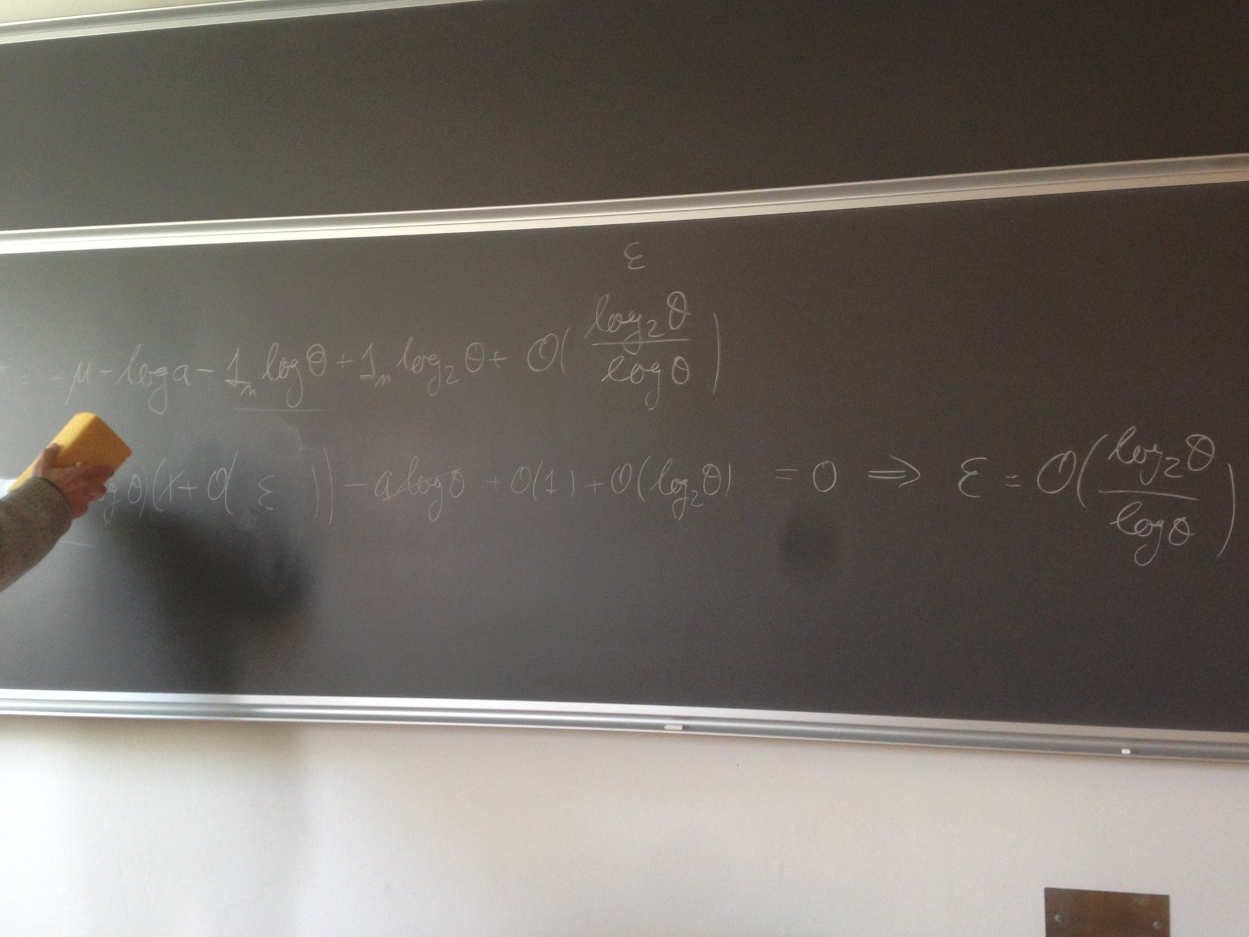
x_i^* \sim \sum_{j=1}^d \beta_{i,j} \log_j t - \mu_i + c_i
\log_1(x) \equiv \log(x) \text{ and } \log_n(x) \equiv \log(\log_{n-1}(x))

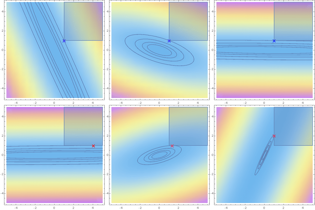
Savage condition

\text{minimise } x^\top \Sigma^{-1} x \text{ under the linear constraint } x \ge 1
\text{Savage condition} \equiv \Sigma^{-1} 1 > 0

Hashorva, E. (2005), 'Asymptotics and bounds for multivariate Gaussian tails', Journal of Theoretical Probability

Laplace's method

\int_a^b \mathrm{e}^{ t f(x) } \, \mathrm{d} x \quad \text{as} \quad t \to \infty

Find  

x^* = \mathrm{arg\,max}_x f(x)

Expand with 2nd order Taylor series about the maximiser

\int_a^b \mathrm{e}^{ t f(x) } \, \mathrm{d} x \approx \mathrm{e}^{ t f(x^*) } \int_{-\infty}^{\infty} \mathrm{e}^{ -t | f''(x^*) | \frac{(x-x^*)^2}{2} } \, \mathrm{d} x
\int_a^b \mathrm{e}^{ t f(x) } \, \mathrm{d} x \approx \sqrt{ \frac{ 2 \pi }{ t | f''(x^*) | } } \mathrm{e}^{ t f(x^*) }

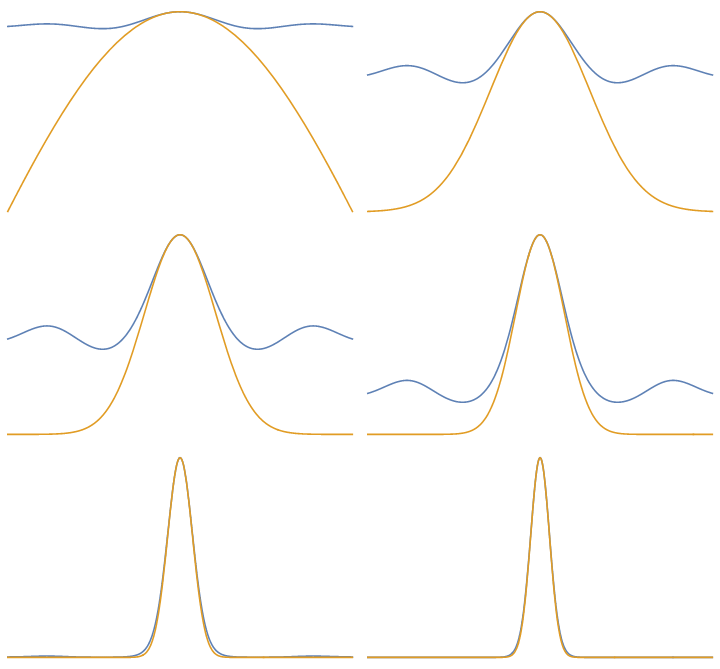
Example

f(x) = \sin(x) / x
\mathrm{e}^{ t f(x) } \text{ is blue and } \mathrm{e}^{ t f(x^*) -t | f''(x^*) | \frac{(x-x^*)^2}{2} } \text{ is orange}

Orthogonal polynomial expansions

  1. Choose a reference distribution, e.g,
\nu = \mathsf{Gamma}(r,m) \Rightarrow f_\nu(x) \propto x^{r-1}\mathrm{e}^{-\frac{x}{m}}

2. Find its orthogonal polynomial system

\{ Q_n(x) \}_{n\in \mathbb{N}_0}
f_X(x) = f_\nu(x) \times \sum_{k=0}^\infty q_k Q_k(x)

3. Construct the polynomial expansion

Pierre-Olivier Goffard

Asmussen, S., Goffard, P. O., & Laub, P. J. (2017). Orthonormal polynomial expansions and lognormal sum densities. Risk and Stochastics - Festschrift for Ragnar Norberg (to appear).

Orthogonal polynomial systems
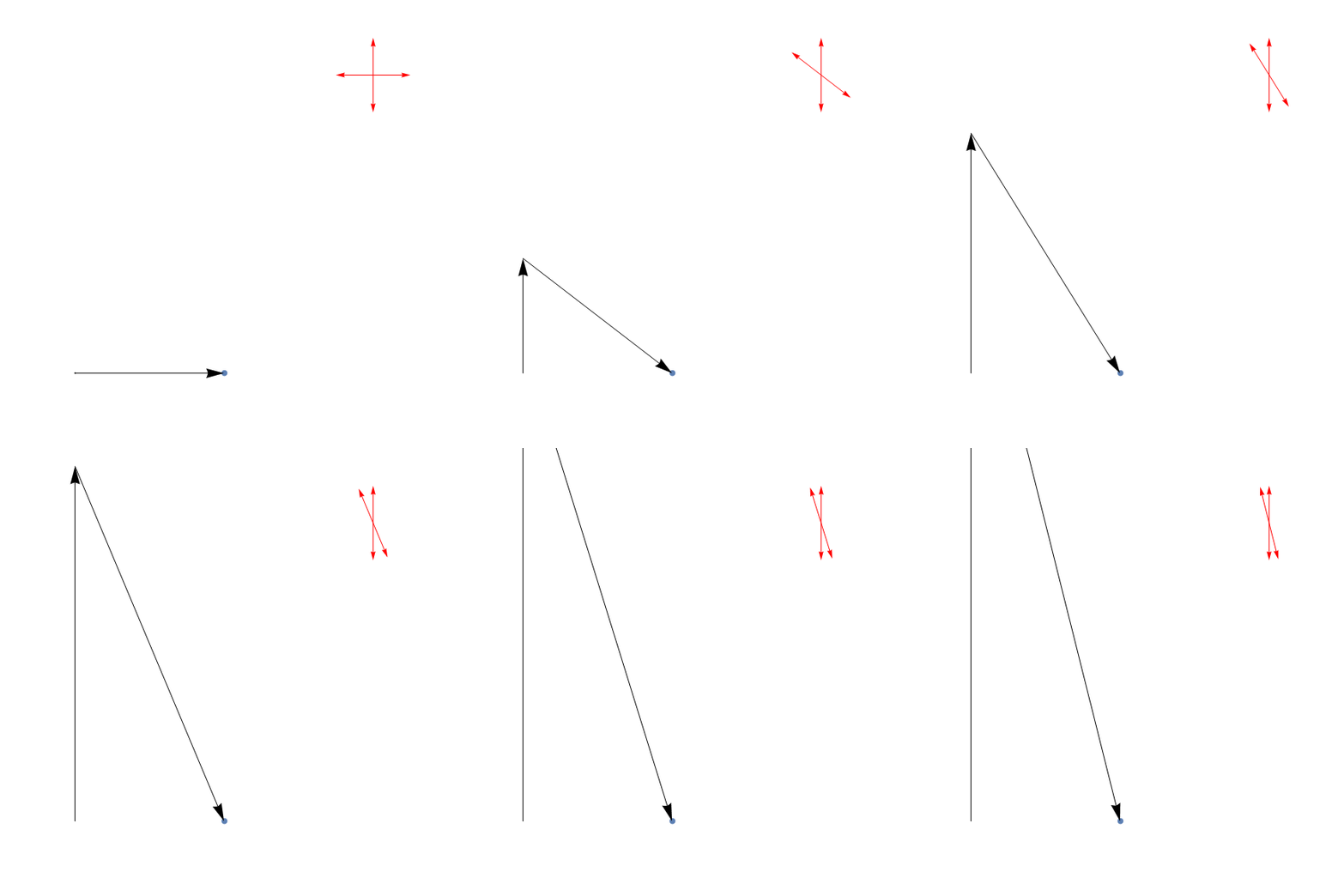
\langle Q_i, Q_j \rangle_\nu = \int Q_i(x) Q_j(x) f_\nu(x) \mathrm{d} x = \begin{cases} 1 & \text{if } i=j \\ 0 & \text{otherwise} \end{cases}

Example: Laguerre polynomials

f_\nu(x) \propto x^{r-1}\mathrm{e}^{-\frac{x}{m}}
L_{n}^{r-1}(x)=\sum_{i=0}^{n} \binom{n + r - 1}{n - i} \frac{(-x)^i}{i!}
Q_n(x) \propto L_n^{r-1}(x/m)

If the reference is Gamma 


then the orthonormal system is 

Q_0(x) = 1 \quad Q_1(x) = x - 1
Q_2(x) = \frac12 x^2 - 2 x + 1 \quad \ldots

For r=1 and m=1,

Final steps

f_X(x) = f_\nu(x) \times \sum_{k=0}^\infty q_k Q_k(x) \Leftrightarrow \frac{f_X(x)}{ f_\nu(x) } = \sum_{k=0}^\infty q_k Q_k(x)
f_X(x) \approx f_\nu(x) \times \sum_{k=0}^K q_k Q_k(x)
q_k = \langle \frac{f_X}{f_\nu} , Q_k \rangle_\nu = \int Q_k(x) f_X(x) \mathrm{d}x = \mathbb{E}[ Q_k(X) ]

Final final step: cross fingers & hope that the q's get small quickly...

Calculating the coefficients

1. From the moments


2. Monte Carlo Integration

q_k \approx \frac1R \sum_{r=1}^R Q_k(X_r)
X_1, X_2, \ldots, X_R \sim f_X
q_k = \mathbb{E}[ Q_k(X) ]
\text{E.g.}~Q_2(x) = \frac12 x^2 - 2 x + 1 \text{ so }
q_2 = \mathbb{E}[\frac12 X^2 - 2 X + 1] = \frac12\mathbb{E}[X^2] - 2 \mathbb{E}[X] + 1

3. (Dramatic foreshadowing) Taking  derivatives of the Laplace transform...

Applied to sums

\text{Want } f_S \text{ where } S \sim \mathsf{LognormalSum}(\mu, \Sigma)


  • Moments


  • Monte Carlo Integration


  • Taking  derivatives


  • Gauss Quadrature
q_k \approx \frac1R \sum_{r=1}^R Q_k(S_r)
S_1, S_2, \ldots, S_R \sim f_S
\text{Requires } \mathscr{L}_S(t)
\mathbb{E}[S] = \mathbb{E}[X_1]+\ldots+\mathbb{E}[X_d]
\mathbb{E}[S^2] = \sum_{i=0}^n \mathbb{E}[X_i^2] + 2 \sum_{i < j} \mathbb{E}[ X_i X_j ]
q_k = \int_{\mathbb{R}_+} Q_k(s) f_S(s) \mathrm{d}s = \int_{\mathbb{R}_+^d} Q_k( 1 \cdot \mathrm{e}^{x}) f_X(x) \mathrm{d}x

Title Text

Subtitle

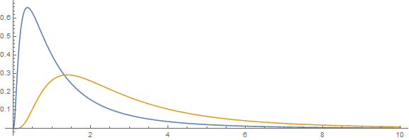
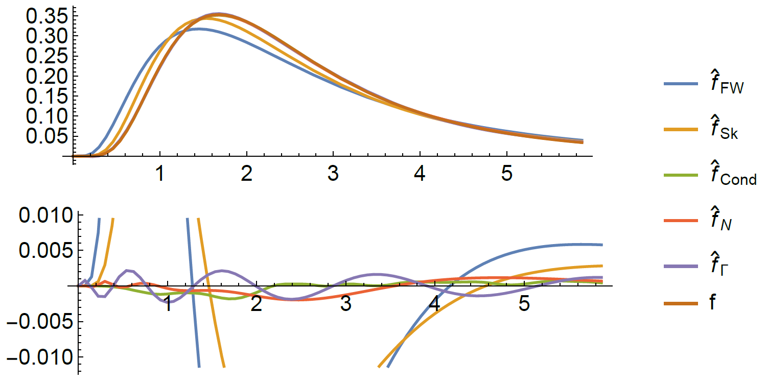
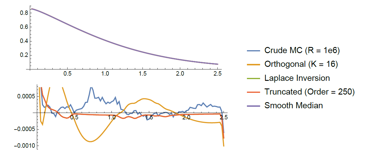
\mu = (0, 0), ~ \mathrm{diag}(\Sigma) = (0.5, 1), ~ \rho = -0.2, ~ K = 32, 16.

An example test

Applications to option pricing

f_S(x) \approx f_\nu(x) \times \sum_{k=0}^K q_k Q_k(x)
\mathbb{E}[ (S - a)_+ ] = \ldots

Dufresne, D., & Li, H. (2014).

'Pricing Asian options: Convergence of Gram-Charlier series'.

Goffard, P. O., & --- (2017). 'Two numerical methods to evaluate stop-loss premiums'. Scandinavian Actuarial Journal (submitted).

S = X_1 + \ldots + X_N

Extension to random sums

Say you don't know how many summands you have...

Imagine you are an insurance company;

there's a random amount of accidents to pay out (claim frequency),

and each costs a random amount (claim size)

Approximate S using orthogonal polynomial expansion

A simplification

= \sum_{i=0}^{\infty} p_i \gamma(r+i,m,x)
\gamma(\alpha,\beta,x) = \text{PDF}(\mathsf{Gamma}(\alpha,\beta), x)
f_{X}(x)=\sum_{k=0}^{\infty} q_k Q_{k}(x) f_\nu(x)

where

p_i = \sum_{k=i}^\infty q_k (-1)^{i+k} \binom{k}{i}
\text{and } p_i \text{ depends on the } q_k's \text{ and } r. \text{ For } r=1,
\overline{F}_{X}(x) = \sum_{i=0}^{\infty}p_i\overline{\Gamma}(r+i,m,x)
\mathbb{E}\left[\left(X-a\right)_{+}\right] = \int_{a}^\infty x f_X(x) \mathrm{d} x - a \overline{F}_X(a)
f_{X}(x)= \sum_{i=0}^{\infty} p_i \gamma(r+i,m,x)
= \sum_{i=0}^{\infty}p_i m (r+i) \overline{\Gamma}(r+i+1,m,a)-a\overline{F}_{X}(a)

The stuff we want to know

As


and using

we can write

\overline{\Gamma}(r,m,x) \equiv \int_{x}^\infty \gamma(r,m,x) \mathrm{d} x

Laplace transform of random sum

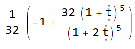
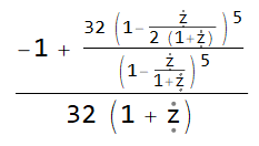
\mathcal{Q}(z) \equiv \sum_{k=0}^\infty q_k c_k z^k = (1+z)^{-r} \mathscr{L}_{S_N}\big( \frac{-z}{m(1+z)} \big)
q_k = \frac{1}{c_k \times k! }\frac{\mathrm{d}^{k}}{\mathrm{d} z^{k}} \mathcal{Q}(z)\Big|_{z=0}
\mathscr{L}_{S_N}(t) = \mathcal{G}_N ( \mathscr{L}_X(t) )
\mathcal{G}_N(z) \equiv \mathbb{E}[z^N]

With                                   we can deduce

and just take derivatives
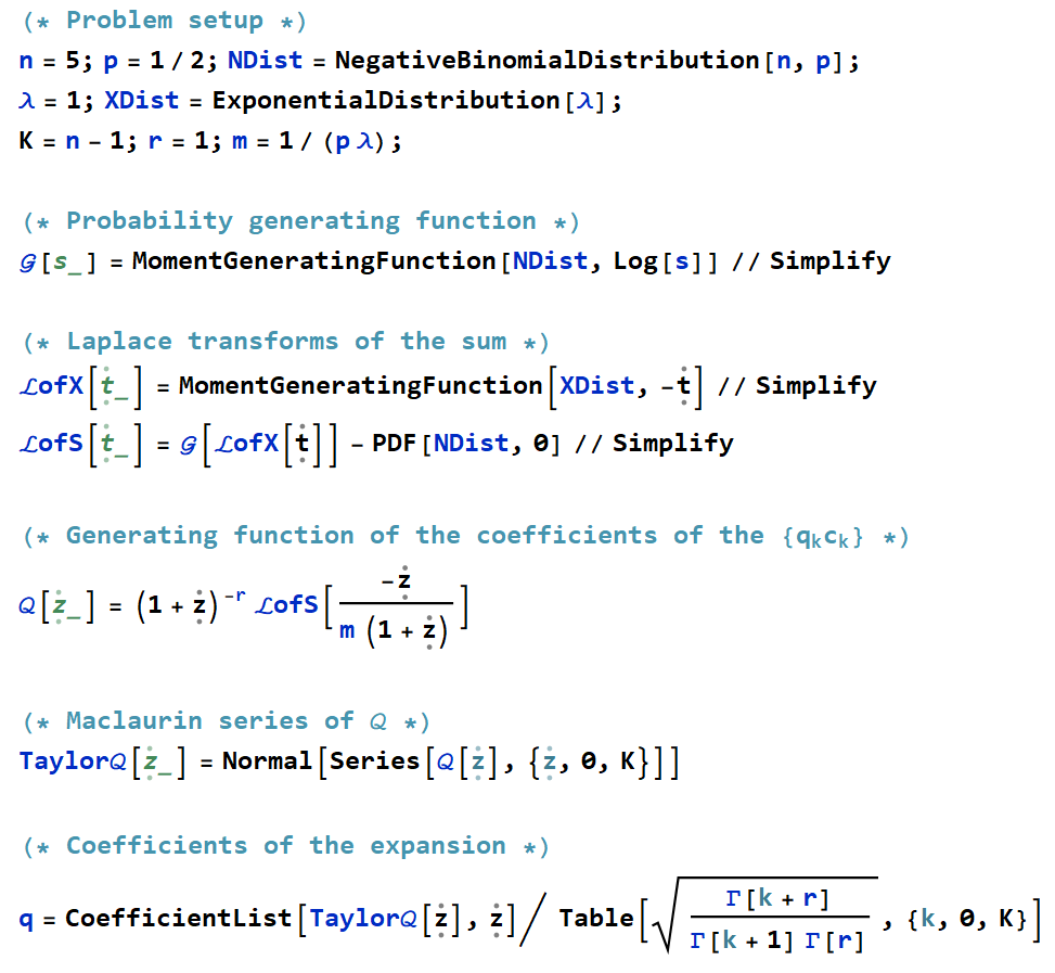
\text{then we get the gen. function of } \{ q_k c_k\}_{k \in \mathbb{N}_0} \text{ where } c_k = \sqrt{\frac{\Gamma(k+r)}{\Gamma(k+1)\Gamma(r)}}

Another example test

N\sim\mathsf{Poisson}(\lambda=2) \text{ and } U\sim\mathsf{Gamma}(r=3/2,m=1/3)

Other things I don't have time to talk about

  • Andersen, L.N., ---, Rojas-Nandayapa, L. (2017) ‘Efficient simulation for dependent rare events with applications to extremes’. Methodology and Computing in Applied Probability
  • Asmussen, S., Hashorva, E., --- and Taimre, T. (2017) ‘Tail asymptotics of light-tailed Weibull-like sums’. Polish Mathematical Society Annals.

In progress:

  • Taimre, T., ---, Rare tail approximation using asymptotics and polar coordinates
  • Salomone, R., ---, Botev, Z.I., Density Estimation of Sums via Push-Out, Mathematics and Computers in Simulation
  • Asmussen, S., Ivanovs, J., ---, Yang, H., 'A factorization of a Levy process over a phase-type horizon, with insurance applications

Thomas Taimre

Robert Salomone

Thanks for listening!

and a big thanks to UQ/AU/ACEMS for the $'s

And thanks to my supervisors

Rare-event asymptotics and estimation for dependent random sums – an exit talk, with applications to finance and insurance

By plaub

Rare-event asymptotics and estimation for dependent random sums – an exit talk, with applications to finance and insurance

  • 2,640