NumPy
佛倫斯
Numerical Python
prerequisite (n.)
先決條件
下載matplotlib
NumPy官方說一定要下載matplotlib
所以我們就照以下步驟下載吧!
Windows 命令提示字元
pip install matplotlib
Mac 終端機
pip3 install matplotlib
下載完matplotlib後
進去Python Shell
import matplotlib
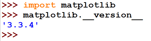
都是兩個底線
若不幸失敗的話
就用 repl 吧,它真的不會有問題

我們開始吧!
NumPy是什麼?
NumPy(Numerical Python)是Python語言的一個擴展程序庫,支持大量的維度數組與矩陣運算,此外也針對數組運算提供大量的數學函數庫。
反正他跟數學有關
應該不會是什麼善良的東西

建立一維陣列
import numpy as np
# 這樣numpy.array只要打np.array就好了
# 可以打比較少字。不是佛倫斯懶惰,
# 是網路上真的都這樣打

a = np.array([1, 2])
print(a)

# output: [1 2]
通常這個陣列裡面都是放數字
因為可以做運算
建立一維陣列
輸入
import numpy as np

a = np.array([1, 2])
print(a)

q = [1, 2]
print(q)

b = np.array(q)
print(b)

print(type(a))
print(type(q))
print(type(b))
# [1 2]
# [1, 2]
# [1 2]
# <class 'numpy.ndarray'>
# <class 'list'>
# <class 'numpy.ndarray'>輸出
陣列元素可用
list傳入
建立一維陣列
輸入
import numpy as np

a = np.array([1, 2])
print(a)

p = (1, 2)
print(p)

b = np.array(p)
print(b)

print(type(a))
print(type(p))
print(type(b))
# [1 2]
# (1, 2)
# [1 2]
# <class 'numpy.ndarray'>
# <class 'tuple'>
# <class 'numpy.ndarray'>輸出
陣列元素可用
tuple傳入
建立二維陣列
輸入
import numpy as np

a = np.array([[0, 1], [1, 0]])
print(a)

q = [[0,1],[1,0]]
print(q)

b = np.array(q)
print(b)

print(type(a))
print(type(q))
print(type(b))
# [[0 1]
# [1 0]]
# [[0, 1], [1, 0]]
# [[0 1]
# [1 0]]
# <class 'numpy.ndarray'>
# <class 'list'>
# <class 'numpy.ndarray'>輸出
陣列元素可用
list傳入
建立二維陣列
輸入
import numpy as np

a = np.array([[0, 1], [1, 0]])
print(a)

p = ((0,1),(1,0))
print(p)

b = np.array(p)
print(b)

print(type(a))
print(type(p))
print(type(b))
# [[0 1]
# [1 0]]
# ((0, 1), (1, 0))
# [[0 1]
# [1 0]]
# <class 'numpy.ndarray'>
# <class 'tuple'>
# <class 'numpy.ndarray'>輸出
陣列元素可用
tuple傳入
其實也可以建三維陣列
只是我真的不知道能幹嘛用
所以下面這個就給大家參考看看就好
import numpy as np
a = np.zeros((2, 2, 3), dtype=int)
print(a)

# 輸出:
# [[[0 0 0]
#   [0 0 0]]

#  [[0 0 0]
#   [0 0 0]]]
np.zeros(), dtype是什麼東西
待會解釋
2×2×3的陣列
更改資料
import numpy as np

a = np.array([[0, 1], [1, 0]])
v = np.array((0, 1))

a[0][0] = 6
v[0] = 9

print(a)
print(v)

# 輸出:
# [[6 1]
#  [1 0]]
# [9 1]
ndarray的孩子們
import numpy as np

a = np.array([[0, 1, 0], [1, 0, 1]])

# a是幾維陣列
print(a.ndim)
# 中括號幾層就是幾維

# a是幾乘幾的陣列
print(a.shape)

# a裡面有幾個元素
print(a.size)

# 輸出:
# 2
# (2, 3)
# 6
dimensional (n.) 維度
我們說這是2×3的陣列,2列3行
小測驗
import numpy as np

a = np.array([[0, 1, 0], [1, 0, 1]])
b = np.array([0, 1, 2, 3, 4, 5, 6])

if (a.ndim > b.ndim):
  print('A', end='')
else:
  print('B', end='')

if (a.size <= b.size):
  print('VHOW')
else:
  print('WEVOH')
請問應該輸出什麼?
import numpy as np

a = np.array([[0, 1, 0], [1, 0, 1]])
b = np.array([0, 1, 2, 3, 4, 5, 6])

# a.ndim = 2, b.ndim = 1
if (a.ndim > b.ndim):
  print('A', end='')
else:
  print('B', end='')
# output: A

# a.size = 6, b.size = 7
if (a.size <= b.size):
  print('VHOW')
else:
  print('WEVOH')
# output: VHOW

# 輸出:
# AVHOW
010笑死
import numpy as np

lorence = np.zeros(6)
forence = np.ones(6)
florence = np.zeros((3, 3), dtype=int)

print(lorence)
print(forence)
print(florence)

# 輸出:
# [0. 0. 0. 0. 0. 0.]
# [1. 1. 1. 1. 1. 1.]
# [[0 0 0]
#  [0 0 0]
#  [0 0 0]]
zero的複數的確是zeros
不是zeroes
那個點很煩
所以宣告它的dtype是int
它們就是整數就不會有點
使用arange建立一維陣列
import numpy as np
royalex = np.arange(9)
dot_line = np.arange(0, 10, 2)
penghc = np.arange(69, 60, -2)
print(royalex)
print(dot_line)
print(penghc)

# 規則跟range一樣

# 輸出:
# [0 1 2 3 4 5 6 7 8]
# [0 2 4 6 8]
# [69 67 65 63 61]

# 記住,若R = np.arange(a, b, c)
# R裡不會有元素b
arange配reshape
建立二維陣列
3列5行
2列4行
import numpy as np

a = np.arange(15).reshape(3, 5)
v = np.arange(0, 40, 5).reshape(2, 4)

print(a)
print(v)

# 輸出:
# [[ 0  1  2  3  4]
#  [ 5  6  7  8  9]
#  [10 11 12 13 14]]
# [[ 0  5 10 15]
#  [20 25 30 35]]
看他印出來長
什麼樣子就知道了
3×5
2×4
小測驗
import numpy as np

avhow = np.array(69, 87, 1).reshape(3, 6)
print(avhow[2][1])
求輸出
import numpy as np

avhow = np.array(69, 87, 1).reshape(3, 6)
print(avhow[2][1])
\(69+6\times 2+1=82\)
# [[69 70 71 72 73 74]
#  [75 76 77 78 79 80]
#  [81 82 83 84 85 86]]
從 \(69\) 往下走兩格加兩次 \(6\)
再往右走一格加 \(1\)
解答
使用linspace建立陣列
import numpy as np
x = np.linspace(0, 2, 9)
# 把0~2切成9-1=8等份,然後頭尾都印出,所以會輸出9數
y = np.linspace(0, 8, 11)
# 把0~8切成10等份,頭尾都輸出,共輸出11數
print(x)
print(y)

# 輸出:
# [0.   0.25 0.5  0.75 1.   1.25 1.5  1.75 2.  ]
# [0.  0.8 1.6 2.4 3.2 4.  4.8 5.6 6.4 7.2 8. ]
np.linspace(x, y, z)要切幾等分的問題可以想想種樹問題
8棵樹會有7個間隔,所以如果要切7份就要在z處填8
小測驗
求x裡面所有元素的和
import numpy as np
x = np.linspace(-3.22, 9.22, 100)
小測驗
\(\displaystyle \frac{9.22+(-3.22)}{2}\times 100=300\)
\(-3.22\sim 9.22\) 切 \(99\) 「等」分,
直接用等差中項 \(\times\) 項數
import numpy as np
x = np.linspace(-3.22, 9.22, 100)
向量、矩陣運算
以下內容會可能引起不適
請大家不要害怕
會涵括高中第3A、4A冊數學內容
還不會的人
不要擔心
佛倫斯原本也不會(或忘光)這些東西
備課前才在看這些
我們在一樣的基礎上學習
向量(Vector)
一維陣列
因為我們國中都有學過笛卡爾直角坐標
下一頁的例子看一看就會了
但是平面向量絕對不只有今天教的這些
請期待高二的數學課~
\(\newcommand{\longvec}[1]{\stackrel\longrightarrow{\smash{#1}\vphantom{i}}} \longvec{AB} \ = (3,3)\) 或 \(3\vec{i}+3\vec{j}\) 或 \(\begin{bmatrix}3 \\3\end{bmatrix}\)
x
y
平面向量
其中 \(\vec{i}\) 表示 \(x\) 軸方向的單位向量,
即 \((1, 0)\) 或 \(\begin{bmatrix}1 \\ 0\end{bmatrix}\)
\(\vec{j}\) 表示 \(y\) 軸方向的單位向量,
即 \((0, 1)\) 或 \(\begin{bmatrix}0 \\ 1\end{bmatrix}\)
\(\newcommand{\longvec}[1]{\stackrel\longrightarrow{\smash{#1}\vphantom{i}}} \longvec{AB}\ =(3, 3)\) 表示從 \(A\) 到 \(B\) 要往 \(x\) 方向走 \(3\) 單位,再往 \(y\) 方向走 \(3\) 單位。
也就是 \(B\) 點座標減掉 \(A\) 點座標(終點減起點)
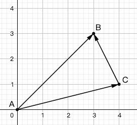
\(A = (0, 0),\ B = (3, 3),\ C = (4, 1)\)
x
y
平面向量
\(\newcommand{\longvec}[1]{\stackrel\longrightarrow{\smash{#1}\vphantom{i}}} \longvec{AB}\ =(3, 3)\)
\(\newcommand{\longvec}[1]{\stackrel\longrightarrow{\smash{#1}\vphantom{i}}} \longvec{AC}\ =(4, 1)\)
\(\newcommand{\longvec}[1]{\stackrel\longrightarrow{\smash{#1}\vphantom{i}}} \longvec{CB}\ =B\) 座標\(-C\) 座標
\(=(3, 3)-(4, 1)=(-1, 2)\)
\(\newcommand{\longvec}[1]{\stackrel\longrightarrow{\smash{#1}\vphantom{i}}} \longvec{AB}\ =\ \longvec{AC}+\longvec{CB}\)
從 \(A\) 走到 \(C\),再從 \(C\) 走到 \(B\),就等於從 \(A\) 走到 \(B\)
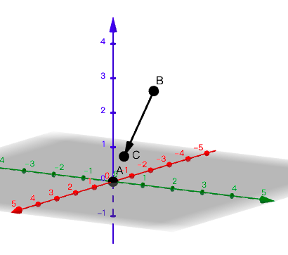
\(A=(0, 0, 0)\)
\(B=(1, 2, 3)\)
\(C=(1, 1, 1)\)
\(\newcommand{\longvec}[1]{\stackrel\longrightarrow{\smash{#1}\vphantom{i}}} \longvec{AB} \ = (1, 2, 3)\)
\(\newcommand{\longvec}[1]{\stackrel\longrightarrow{\smash{#1}\vphantom{i}}} \longvec{AC} \ = (1, 1, 1)\)
\(\newcommand{\longvec}[1]{\stackrel\longrightarrow{\smash{#1}\vphantom{i}}} \longvec{BC} \ = (0, -1, -2)\)
\(\newcommand{\longvec}[1]{\stackrel\longrightarrow{\smash{#1}\vphantom{i}}} \longvec{AC}\ =\ \longvec{AB}+\longvec{BC}\)
空間向量
這張圖其實根本沒用,因為螢幕是平面的
x
y
z
向量加法、減法
x座標加(減)x座標
y座標加(減)y座標
z座標加(減)z座標
例:\(\vec{u} = (2, 3, 3),\ \vec{v}=(-4, -2, 0)\)
\(\vec{u}+\vec{v}=(2+(-4),\ 3+(-2),\ 3+0)=(-2,\ 1,\ 3)\)
\(\vec{u}-\vec{v}=(2-(-4),\ 3-(-2),\ 3-0)=(6,\ 5,\ 3)\)
用numpy操作向量加、減法
import numpy as np
AB = np.array([3,3])
AC = np.array([4,1])
CB = AB-AC
print(CB)
print(AC+CB)

# 輸出:
# [-1  2]
# [3 3]
\(\newcommand{\longvec}[1]{\stackrel\longrightarrow{\smash{#1}\vphantom{i}}} \longvec{AB} \ = (3,3)\)
\(\newcommand{\longvec}[1]{\stackrel\longrightarrow{\smash{#1}\vphantom{i}}} \longvec{AC} \ = (4,1)\)
\(\newcommand{\longvec}[1]{\stackrel\longrightarrow{\smash{#1}\vphantom{i}}} \longvec{CB}\ =\ \longvec{AB}-\longvec{AC}=(3, 3)-(4, 1)=(-1, 2)\)
\(\newcommand{\longvec}[1]{\stackrel\longrightarrow{\smash{#1}\vphantom{i}}}\longvec{AC}+\longvec{CB}\ =(4, 1)+(-1, 2)=(3, 3)=\ \longvec{AB}\)
向量乘上一個常數
\(\alpha (a, b, c)=(\alpha a, \alpha b, \alpha c)\)
例:\(\vec{v} = (1, 4),\ \vec{w} = 4\vec{v} =(4\times 1,\ 4\times 4) = (4, 16)\)
\(\vec{a}=(6, 9, 6),\ \vec{b}=\frac{1}{3}\vec{a}=(2, 3, 2)\)
import numpy as np
v = np.array([1, 4])
w = 4*v
a = np.array([6, 9, 6])
b = a/3
print(w)
print(b)

# 輸出:
# [ 4 16]
# [2. 3. 2.]
向量的大小(絕對值)
例:\(\vec{v}=(1, 2),\ \vec{w}=(2, 1, 2)\)
\(|\vec{v}|\) 其實就是 \(\vec{v}\) 的長度
\(|\vec{v}|=\sqrt{1^2+2^2}=\sqrt{5}\)
\(|\vec{w}|=\sqrt{2^2+1^2+2^2}=\sqrt9=3\)
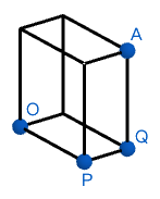
\(OQ=\sqrt{OP^2+PQ^2}\)
\(AQ\) 垂直 \(OPQ\) 平面
\(OQ\perp OA\implies OA=\sqrt{OQ^2+AQ^2}\)
\(\implies OA=\sqrt{OP^2+OQ^2+QA^2}\)
向量應用
以下內容牽涉選修物理課程,可能引發部分人的不適
但是沒關係,佛倫斯也不會物理
佛倫斯物理考過0分
向量應用
以下內容牽涉選修物理課程,可能引發部分人的不適
已知:\(\vec{v}=\vec{v_0}+\vec{a}t\)
速率 = 速度的絕對值
\(\vec{v}\) 代表末速、\(\vec{v_0}\) 代表初速、\(\vec{a}\) 代表加速度、\(t\) 代表時間
若一個質點初速 \(\vec{v_0}=(-4697, -822)\)
加速度 \(\vec{a}=(10, 37)\)
試問過了 \(t=69\) 秒質點的
(1) 速度為何? (2) 速率為何?
import numpy as np
import math
v0 = np.array([-4697, -822])
a = np.array([10, 37])
t = 69
v = v0 + a*t
print(v)
print(math.sqrt(v[0]*v[0]+v[1]*v[1]))

# 輸出:
# [-4007  1731]
# 4364.906642758811
\(\vec{v}=\vec{v_0}+\vec{a}t\)
\(|\vec{v}|=\sqrt{(-4007)^2+1731^2}\)
習題(一)
一質量為 \(m\) 的質點在「空間」中運動,其初速為 \(\vec{v_0}\)。質點受到一衝量 \(\vec{J}\) 後,新的速度為 \(\displaystyle \vec{v}=\vec{v_0}+\frac{\vec{J}}{m}\)
給定該質點的質量、初速、末速
(照順序,數字皆為整數)
求衝量 \(\vec{J}\)。
注意!是在空間運動。一維陣列裡面要有三個元素!
如何在同一行輸入多個整數
a, b, c = map(int, input().split())照上面那一行打就可以在一行內輸入多個以空格隔開的整數
習題(一)
範例輸出:
[2 4 4]
範例輸入:
2
0 0 0
1 2 2
\(m\)
\(\vec{v_0}\)
\(\vec{v}\)
接下來時間給大家練習
習題(一)
習題(一)解答
\(\displaystyle \vec{v}=\vec{v_0}+\frac{\vec{J}}{m}\)
移項
\(\vec{J}=m(\vec{v}-\vec{v_0})\)
import numpy as np
m = int(input())
vx0, vy0, vz0 = map(int, input().split())
v0 = np.array([vx0, vy0, vz0])
vx, vy, vz = map(int, input().split())
v = np.array([vx, vy, vz])
J = m*(v-v0)
print(J)
矩陣(Matrix)
二維陣列
** matrix的複數是matrices **
\(\begin{bmatrix}a_{11} & a_{12} & a_{13} & \cdots & a_{1n} \\ a_{21} & a_{22} & a_{23} & \cdots & a_{2n} \\ \vdots & & \ddots & & \\ a_{m1} & a_{m2} & a_{m3} & \cdots & a_{mn}\end{bmatrix}\)
\(n\) 行
\(m\) 列
這是一個 \(m\times n\) 階的矩陣
\(A=[a_{ij}]_{m\times n}\ \ (1\leq i\leq m,\ 1\leq j\leq n)\)
怕搞混行和列的話,還記得前面的shape嗎?
所以記好了!m×n階的矩陣代表它有m列n行,
不要再背反了
import numpy as np
A = np.ones((4, 2), dtype=int)
B = np.ones((2, 4), dtype=int)
print(A, B, sep='\n')

# 輸出:
# [[1 1]
#  [1 1]
#  [1 1]
#  [1 1]]
# [[1 1 1 1]
#  [1 1 1 1]]
(4, 2)
代表 \(A\) 就是4×2階的矩陣
印出來發現是4列2行
(2, 4)
代表 \(B\) 就是2×4階的矩陣
印出來發現是2列4行
怕搞混行和列的話,還記得前面的shape嗎?
m×n階的矩陣代表它有m列n行
A.shape是(3, 4),代表A是3×4的矩陣
印出來是3列4行
B.shape是(4, 3),代表B是4×3的矩陣
印出來是4列3行
import numpy as np
A = np.array([[2, 3, 5, 7], [11, 13, 17, 19],
              [23, 29, 31, 37]])
B = np.arange(2, 38, 3).reshape(4, 3)
print(A)
print(A.shape)
print()
print(B)
print(B.shape)

# 輸出:
# [[ 2  3  5  7]
#  [11 13 17 19]
#  [23 29 31 37]]
# (3, 4)
#
# [[ 2  5  8]
#  [11 14 17]
#  [20 23 26]
#  [29 32 35]]
# (4, 3)
\(A=\begin{bmatrix}2&3&5&7\\11&13&17&19\\23&29&31&37\end{bmatrix}\)
\(B=\begin{bmatrix}2&5&8\\11&14&17\\20&23&26\\29&32&35\end{bmatrix}\)
矩陣加法、減法
\(A,\ B\) 是 \(m\times n\) 階的矩陣
\(A=[a_{ij}]_{m\times n}\)
\(B=[b_{ij}]_{m\times n}\)
\((1\leq i\leq m,\ 1\leq j\leq n)\)
\(A+B=[a_{ij}+b_{ij}]_{m\times n}\)
\(A-B=[a_{ij}-b_{ij}]_{m\times n}\)
上面那些是從數學課本抄來的
看不懂上面數學表示法可以參考下頁的例子
兩矩陣行數列數都要一樣相加/減才有意義
A.shape = B.shape = (m, n)
矩陣加法、減法
\(A=\begin{bmatrix}1 & 2 \\ 3 & 4\end{bmatrix}\),\(B=\begin{bmatrix}-8 & -7 \\ -6 & -5\end{bmatrix}\)
\(A+B = \begin{bmatrix}1+(-8) & 2+(-7) \\ 3+(-6) & 4+(-5)\end{bmatrix}=\begin{bmatrix}-7 & -5 \\ -3 & -1\end{bmatrix}\)
\(A-B = \begin{bmatrix}1-(-8) & 2-(-7) \\ 3-(-6) & 4-(-5)\end{bmatrix}=\begin{bmatrix}9 & 9 \\ 9 & 9\end{bmatrix}\)
\(A, B\) 的行數、列數都是 \(2\),
我們稱它們為「二階方陣」
矩陣加法、減法
在很前面有提到
向量也可以用矩陣來表示
\(\vec{u}=(1, 0, 3)=\vec{i}+3\vec{k}=\begin{bmatrix}1 \\ 0 \\ 3\end{bmatrix}\)
\(\vec{v}=(6, -4, -1)=6\vec{i}-4\vec{j}-\vec{k}=\begin{bmatrix}6 \\ -4 \\ -1\end{bmatrix}\)
\(\vec{u}\pm \vec{v}\) 也可以用矩陣的加減法做,會發現跟
向量加減法得到的結果一樣
用numpy操作矩陣加減法
import numpy as np
A = np.arange(-1, -7, -1).reshape(2, 3)
B = np.ones([2, 3], dtype=int)
C = np.array([[1, 4, 9], [0, 3, -8]])
print(A+B, B+A, sep='\n')
print()
print((A+B)+C, A+(B+C), sep='\n')

# 輸出:
# [[ 0 -1 -2]
#  [-3 -4 -5]]
# [[ 0 -1 -2]
#  [-3 -4 -5]]
#
# [[  1   3   7]
#  [ -3  -1 -13]]
# [[  1   3   7]
#  [ -3  -1 -13]]
矩陣加法
遵守結合律
矩陣加法
遵守交換律
\(A=\begin{bmatrix}-1 & -2 & -3 \\ -4 & -5 & -6\end{bmatrix}\)
\(B=\begin{bmatrix}1&1&1\\1&1&1\end{bmatrix}\)
\(C=\begin{bmatrix}1&4&9\\0&3&8\end{bmatrix}\)
shape都是2×3
矩陣係數積
\(A=[a_{ij}]_{m\times n}\Longrightarrow rA=[ra_{ij}]_{m\times n}\)
import numpy as np
v = np.array([1, 4])
A = np.array([[6, 9], [9, 6]])
print(4*v, A/3, sep='\n')

# 輸出:
# [ 4 16]
# [[2. 3.]
#  [3. 2.]]
\(A\) 裡面每項都乘上 \(r\)
運算子:*
警告!
這個不是矩陣乘法!
numpy的「*」運算子
是兩個同行數同列數的矩陣
把同兩矩陣一個位置的元素乘起來放到另一個同行同列的矩陣
就像加減法那樣一個位置對一個位置
但矩陣乘法可沒這麼簡單
不過我們先看「*」運算子的範例
import numpy as np
A = np.array([[2], [0], [9]])
B = np.array([[-2], [-9], [-1]])
print(A*B)

# 輸出:
# [[-4]
#  [ 0]
#  [-9]]
再次聲明!
這個不是矩陣乘法!
矩陣乘法
\(A=[a_{ij}]_{m\times n},\ B=[b_{ij}]_{n\times p}\)
注意!\(A\) 的行數要跟 \(B\) 的列數一樣
相乘才有意義
\(C=AB=[c_{ij}]_{m\times p}\)
其中 \(\displaystyle c_{ij}=\sum_{k=1}^n a_{ik} b_{kj}\)
上面數學式看不懂沒關係
可以直接看下一頁示範
(就說矩陣乘法沒那麼簡單了)
看到
頂真修辭了嗎?
\(A=\begin{bmatrix}5 & 4 & 2 \\ 1 & 3 & 6\end{bmatrix}\ \ 2\times 3\)階
, \(B=\begin{bmatrix}3 & -1 & 0 & 1 \\ 1 & 0 & 1 & 3 \\ 4 & 3 & 2 & 5\end{bmatrix}\ \ 3\times 4\)階
\(C = AB\quad \quad 2\times 4\)階
\(\displaystyle \implies c_{ij}=a_{i1}b_{1j}+a_{i2}b_{2j}+\cdots\)
\(c_{23}=a_{21}b_{13}+a_{22}b_{23}+a_{23}b_{33} \\ =1\times 0+3\times 1+6\times 2=15\)
\(c_{11}=a_{11}b_{11}+a_{12}b_{21}+a_{13}b_{31}\\ =5\times 3+4\times 1+2\times 4=27\)
\(\begin{bmatrix}5 & 4 & 2 \\ 1 & 3 & 6\end{bmatrix}\)
\(\begin{bmatrix}3 & \ \ -1 & \ \ 0 & \ \ \ 1 \\ 1 & \ \ 0 & \ \ 1 & \ \ \ 3 \\ 4 & \ \ 3 & \ \ 2 & \ \ \ 5\end{bmatrix}\)
\(\begin{bmatrix}c_{11} & c_{12} & c_{13} & c_{14} \\ c_{21} & c_{22} & c_{23} & c_{24}\end{bmatrix}\)
\(A\)
\(B\)
\(A=\begin{bmatrix}5 & 4 & 2 \\ 1 & 3 & 6\end{bmatrix}\ \ 2\times 3\)階
\(B=\begin{bmatrix}3 & -1 & 0 & 1 \\ 1 & 0 & 1 & 3 \\ 4 & 3 & 2 & 5\end{bmatrix}\ \ 3\times 4\)階
\(AB=BA\) 正確嗎?
答案是肯定不對
因為 \(BA\) 根本沒有意義
\(B\) 的行數:\(4\),\(A\) 的列數:\(2\)
這兩個數字不一樣,所以相乘沒意義
故矩陣乘法沒有交換律
用numpy操作矩陣乘法
\(A=\begin{bmatrix}1&0\\0&1\end{bmatrix},\quad B=\begin{bmatrix}6&9\\8&7\end{bmatrix}\)
計算 \(AB,\ BA\)
給定兩個二階方陣 \(A, B\)
A的行數 = B的列數 = 2
B的行數 = A的列數 = 2
所以 \(AB, BA\) 都有意義
用numpy操作矩陣乘法「@」
import numpy as np
A = np.array([[1, 0], [0, 1]])
B = np.array([[6, 9], [8, 7]])
print(A, B, A@B, B@A, sep='\n')

# 輸出:
# [[1 0]
#  [0 1]]
# [[6 9]
#  [8 7]]
# [[6 9]
#  [8 7]]
# [[6 9]
#  [8 7]]
怎麼 A@B 和 B@A
輸出結果一樣?
不是沒有交換律?
可以自己算算看
\(\begin{bmatrix}1&0\\0&1\end{bmatrix}\cdot\begin{bmatrix}6&9\\8&7\end{bmatrix}\) 和 \(\begin{bmatrix}6&9\\8&7\end{bmatrix}\cdot\begin{bmatrix}1&0\\0&1\end{bmatrix}\)
答案是不是剛好一樣
閒的話也可以試試
隨便設一個二階方陣 \(X\)
令 \(I =\begin{bmatrix}1&0\\0&1\end{bmatrix}\)
看看 \(X\cdot I,\ I\cdot X\) 是不是一樣
用numpy操作矩陣乘法「@」
不一樣了吧,剛剛那個只是巧合
import numpy as np
A = np.array([[5, 4], [-8, -7]])
B = np.array([[6, 9], [8, 7]])
print(A@B, B@A, sep='\n')

# 輸出:
# [[  62   73]
#  [-104 -121]]
# [[-42 -39]
#  [-16 -17]]
\(A=\begin{bmatrix}5&4\\-8&-7\end{bmatrix}\)
\( B=\begin{bmatrix}6&9\\8&7\end{bmatrix}\)
\(A=\begin{bmatrix}5&4\\-8&-7\end{bmatrix},\quad B=\begin{bmatrix}6&9\\8&7\end{bmatrix}\)
沒事也可以自己練習動手算 \(AB, BA\) 是多少
兩個答案確實不同
習題(二)
給定一個二階方陣 \(A\),試求 \(A\) 的乘法反方陣 \(A^{-1}\)。
設矩陣 \(I=A\cdot A^{-1}\),求 \(I\)。
已知若 \(A=\begin{bmatrix}a & b \\ c & d\end{bmatrix}\),\(\displaystyle A^{-1}=\frac{1}{ad-bc}\begin{bmatrix}d & -b \\ -c & a\end{bmatrix}\)
輸入保證 \(ad\neq bc\)
範例輸入:
1 0
0 1
範例輸出:
[[1. 0.]
[0. 1.]]
[[1. 0.]
[0. 1.]]
import numpy as np
a, b = map(int, input().split())
c, d = map(int, input().split())
A = np.array([[a, b], [c, d]])
B = 1/(a*d-b*c) * np.array([[d, -b], [-c, a]])
I = A@B
print(B, I, sep='\n')

# B就是A的乘法反方陣
習題(二)解答
\(A^{-1}\) 的定義就是一個乘上 \(A\) 會等於 \(\begin{bmatrix}1 & 0 \\ 0 & 1\end{bmatrix}\) 的矩陣
定義 \(I=\begin{bmatrix}1 & 0 \\ 0 & 1\end{bmatrix}\) 為二階單位方陣
習題(二)解答
來簡單驗證一下題目給的 \(A^{-1}\) 的公式是否正確
\(A=\begin{bmatrix}a & b \\ c & d\end{bmatrix},\quad \displaystyle A^{-1}=\frac{1}{ad-bc}\begin{bmatrix}d & -b \\ -c & a\end{bmatrix}\)
\(\displaystyle A\cdot A^{-1}=\begin{bmatrix}a&b\\c&d\end{bmatrix}\cdot \left(\frac{1}{ad-bc}\cdot \begin{bmatrix}d&-b\\-c&a\end{bmatrix}\right)\)
\(\displaystyle = \frac{1}{ad-bc}\cdot\left(\begin{bmatrix}a&b\\c&d\end{bmatrix}\cdot\begin{bmatrix}d&-b\\-c&a\end{bmatrix}\right)\)
\(=\displaystyle \frac{1}{ad-bc}\begin{bmatrix}ad-bc&0\\0&ad-bc\end{bmatrix}\)
\(=\begin{bmatrix}1&0\\0&1\end{bmatrix}\)
其他酷酷的操作
import numpy as np
from numpy import pi
A = np.array([[2, 3, 2], [4, -1, 4], [0, 5, 0]])
print(A**2)
# 把A裡面的每一項都平方再印出來

x = np.linspace(0, 2 * pi, 7)
f = np.sin(x)
print(f)
# sin()是正弦函數,是三角函數的一種

# [[ 4  9  4]
#  [16  1 16]
#  [ 0 25  0]]
# [ 0.00000000e+00  8.66025404e-01
#   8.66025404e-01  1.22464680e-16
#  -8.66025404e-01 -8.66025404e-01
#  -2.44929360e-16]
# 其實e-16那些都是0,電腦出錯了
謝謝大家 <3
今天教的東西只是NumPy的冰山一角而已
因為他是主要是用在數學方面
而我們的基礎還不夠
所以希望大家至少能對今天講的
NumPy向量、矩陣的操作有個印象
如果高二修的是數A,
那麼這些東西很快就會學到了
再過個幾年也許我們就會發現NumPy的強大了
python13
By princetonbxxxh


