Identify Parsimony, Measure Locally, Evaluate Rigorously

Ramchandran Muthukumar

Mentors : Frank Permenter, Chenyang Yuan

Manager : Avinash Balachandran

ML Theory Reading Group

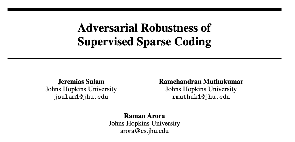
2019

2021

2023

2025

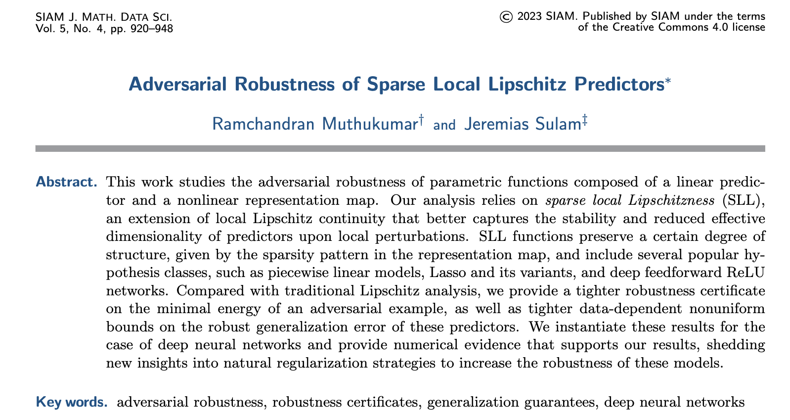
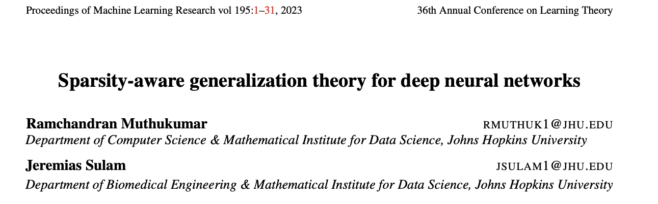
NeurIPS '20

SIAM Journal on
Mathematics of Data Science
(SI-MODS '22)

COLT '23

A theory of generalization
via local parsimony

(under preparation)

Evaluate Rigorously

Identify Parsimony

Roadmap

Measure Locally

Performance of machine learning models

Provable mathematical statements

Evaluate Rigorously

Classification Task

Given an image, classify it

cat

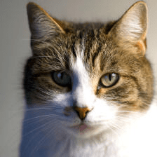
Classification Task

cat

$x$

Input

Label

$ y $

$ \{\textit{cat}, \textit{dog}, \textit{bird}, \ldots \} $

Classify an input in $\mathcal{X}$,
with an appropriate label in $\mathcal{Y}$

$ \mathcal{X}$: images of pets

$ \mathcal{Y}$: types of pets

Some inputs are more common than others

e.g. cats vs pandas

A distribution $ \mathcal{D} $ captures the probability of sampling an input-label pair

Classification Task

$ \mathcal{X}$: images of pets

$ \mathcal{Y}$: types of pets

Classify an input in $\mathcal{X}$,
with an appropriate label in $\mathcal{Y}$

Classification Task

$ \mathcal{X}$: images of pets

$ \mathcal{Y}$: types of pets

Unfortunately $ \mathcal{D} $ is unknown.

For random labeled data $(x,y) \sim \mathcal{D}$,
classify input $x$ as the label $y$

Classify an input in $\mathcal{X}$,
with an appropriate label in $\mathcal{Y}$

$= \{ (x_1, y_1), (x_2, y_2), \ldots (x_m, y_m) \} $

Training Data

Supervised Learning

$ \overset{\mathrm{i.i.d}}{\sim} (\mathcal{D})^m$

$S$

(Proxy)

Does the ability to classify training data $S$,
mean we can also classify data from $\mathcal{D}$ ?

Generalization

when do we generalize?

For training data $(x_i,y_i)$ in $S$,
classify input $x_i$ as the label $y_i$

cat

We search for good models ( ) in a hypothesis class $\mathcal{H}$
$\mathrm{Label}(h,x)$ is the prediction$^*$ of a model $h $ in $ \mathcal{H}$ at input $x$
$\mathrm{margin}(h,(x, y))$ is the margin$^\dagger$ of prediction at a labeled data.
$ \mathrm{margin}(h,(x, y)) > 0 \implies \mathrm{Label}(h,x) = y $

Classification Task

$^*$ $ \mathrm{label}(h, x) \coloneqq \underset{c}{\arg\max}\; [h (x)]_c $

$^\dagger$ $\mathrm{margin}(h,(x, y)) \coloneqq [ h(x)]_{y} - \argmax_{j \neq y} [h(x)]_j$

$x$

$ y $

$ h $

\mathrm{TestError}_{\gamma}(h) =

\mathrm{TrainingError}_{\gamma}(h) = %:= \frac{1}{|\texttt{S}|} \sum_{(x_i, y_i) \text{ in } \texttt{S}} \mathbf{1}\{\mathrm{margin}(h, (x_i, y_i)) < \gamma\}

Fraction$^\star$ of training data
where the margin is insufficient

Probability$^\dagger$ of sampling data
where the margin is insufficient

For $ \gamma = 0 $, $\mathrm{Test Error}_{0}(h) $ is the probability of misclassification

Classification Task

$^\star$ $\mathrm{TrainingError}_{\gamma}(h) := \frac{1}{|\texttt{S}|} \sum_{(x_i, y_i) \text{ in } \texttt{S}} \mathbf{1}\{\mathrm{margin}(h, (x_i, y_i)) < \gamma\}$

$^\dagger$ $\mathrm{TestError}_{\gamma}(h) = \underset{(x, y) \sim \mathcal{D}}{\mathbf{Prob}} \left\{ \mathrm{margin}(h, (x, y)) <\gamma \right\}$

Training samples

Inputs

$ \mathcal{X} \subset \mathbb{R}^d$

Labels

$ \mathcal{Y} := \{1, \ldots, C\} $

Data Distribution

$ \mathcal{D} $ over $ \mathcal{X} \times \mathcal{Y} $ (unknown)

Hypothesis Class

Predicted Label

Margin

$$ \mathrm{label}(h, x) \coloneqq \underset{c}{\arg\max}\; [h (x)]_c$$

$\mathcal{H} : \mathcal{X} \rightarrow \mathbb{R}^C$

$ \texttt{S} := \{ (x_i, y_i) \}_{i=1}^m \overset{\mathrm{i.i.d}}{\sim}$ $(\mathcal{D})^m $

$$\mathrm{margin}( h,( x, y)) \coloneqq [ h(x)]_{y} - \argmax_{j \neq y} [ h(x)]_j $$

Training Error

Test Error

$ \frac{1}{|\texttt{S}|} \sum_{(x_i, y_i) \text{ in } \texttt{S}} \mathbf{1}\{\mathrm{margin}(h, (x_i, y_i)) < \gamma\}$

$ \underset{(x, y) \sim \mathcal{D}}{\mathbf{Prob}} \left\{ \mathrm{margin}(h, (x, y)) <\gamma \right\} $

Classification Task

Does the ability to classify training data $S$,
mean we can also classify data from $\mathcal{D}$ ?

Generalization

when do we generalize?

Classification Task

(Proxy)

For random labeled data $(x,y) \sim \mathcal{D}$,
classify input $x$ as the label $y$

For training data $(x_i,y_i)$ in $S$,
classify input $x_i$ as the label $y_i$

Generalization

when do we generalize?

If $\mathrm{TrainingError}_{\gamma}(h)$ is small,

how large can $\mathrm{Test Error}_{\gamma}(h)$ be?

Classification Task

For random labeled data $(x,y) \sim \mathcal{D}$,
classify input $x$ as the label $y$

For training data $(x_i,y_i)$ in $S$,
classify input $x_i$ as the label $y_i$

(Proxy)

Generalization Bounds

A non-asymptotic, probabilistic bound on the test error of a model

With probability at least $1-\delta$ over the sampling of training data, for any model $h$ in $\mathcal{H}$,

${\bm{\kappa}(\cdot)}$ = capacity measure

valid for any finite training data S of size m

valid with high probability over randomly sampled training data $S \overset{\textrm{i.i.d}}{\sim} (\mathcal{D})^m $

Vacuous if the bound is larger than 1

\mathrm{TestError}_0(h) \leq\mathrm{TrainingError}_{\gamma}(h) + \mathcal{O}\left(\sqrt{\frac{ { \bm{\kappa}(\cdot)}}{m}} +\sqrt{\frac{\log(\frac{1}{\delta})}{m}}\right)

Generalization Bounds

${ \kappa(\cdot)}$ can depend on several things: data distribution $\mathcal{D}$, hypothesis class $\mathcal{H}$, training data $S$, learned model $h$ etc.

How large is $\mathcal{H}$ ?

How expressive is $\mathcal{H}$ on $S$ ?

VC-dimension $\kappa_{\mathrm{VC}}(\mathcal{H})$, Rademacher complexity $\kappa_{\mathrm{RC}}(\mathcal{H}, S)$

\mathrm{TestError}_0(h) \leq\mathrm{TrainingError}_{\gamma}(h) + \mathcal{O}\left(\sqrt{\frac{ { \bm{\kappa}(\cdot)}}{m}} +\sqrt{\frac{\log(\frac{1}{\delta})}{m}}\right)

Generalization Bounds

\mathrm{TestError}_0(h) \leq\mathrm{TrainingError}_{\gamma}(h) + \mathcal{O}\left(\sqrt{\frac{ { \bm{\kappa}(\cdot)}}{m}} +\sqrt{\frac{\log(\frac{1}{\delta})}{m}}\right)

Capacity measures that only depend on $\mathcal{H}$ result in bounds,

1. Uniform over $\mathcal{H}$ - including the bad classifiers
2. Oblivious to learning process

Finding capacity measures that correlate with test error in practice is an active area of research

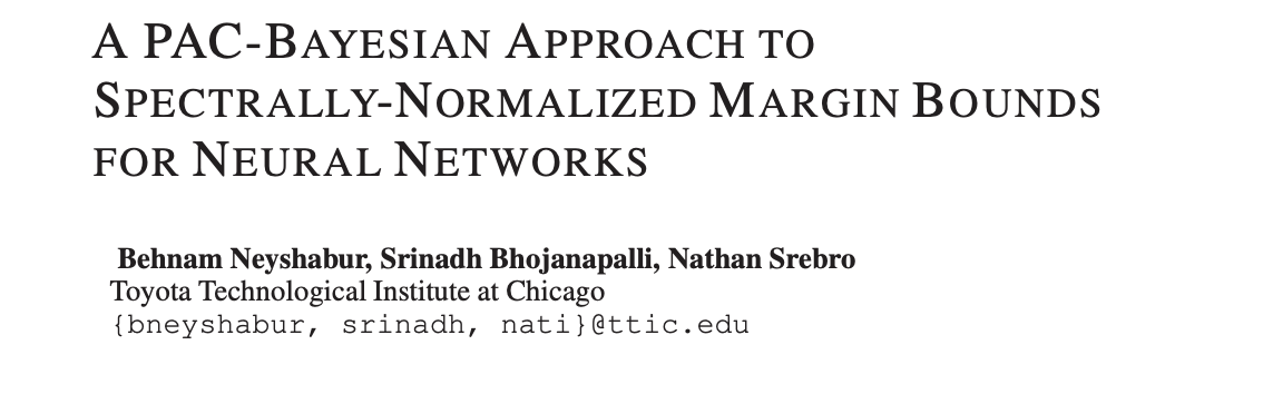
Capacity measures in Deep Learning

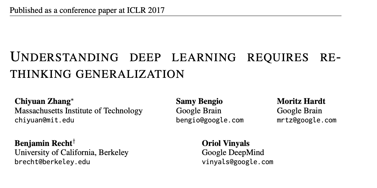
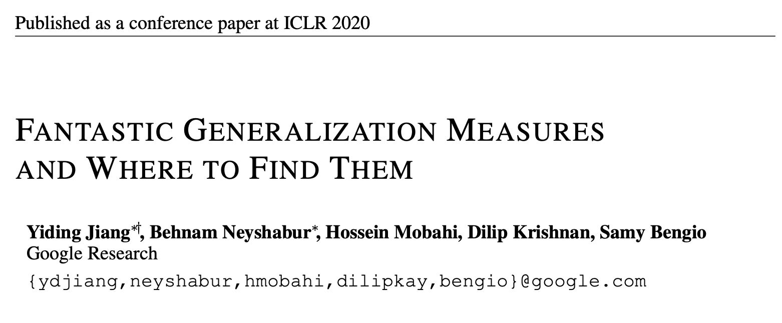
Sensitivity-based capacity

Sensitivity is the rate of change of a model's output under perturbation.
Let $ \mathrm{dist}(\cdot, \cdot)$ be a distance metric over models.
Lipschitz constant $\mathsf{L}_{\rm global}$ is an upper bound on the maximum sensitivity.

For any triple of $(h, x, \hat{h})$, $$\|\hat{h}(x) - h(x) \|_2 \leq \mathsf{L}_{\rm global} \;\mathrm{dist}(\hat{h},h)$$
A larger Lipschitz constant $\mathsf{L}_{\rm global}$ implies the models are more sensitive to perturbations.

global

Generalization via Global Sensitivity

Theorem$^\star$ (Bartlett et. al. (2017), Neyshabur et. al (2017), etc.)

With high probability over the training data S, for any $ h \in \mathcal{H} $

$ \tilde{\mathcal{O}} $ suppresses log factors, constants and failure probability.

$^\star$ Simplified informal statement of results.

Global sensitivity depends on worst-case interaction between the model and data.

Capacity measures that only depend on $\mathcal{H}$ result in uniform bounds

\kappa_{\rm global}(\mathcal{H}) \propto \mathsf{L}_{\rm global}

Can we do better with local information?

$\gamma$ is a hyper-parameter chosen before observing data

\begin{align*} \mathrm{TestError}_0( { h}) &\leq \mathrm{TrainingError}_{\gamma}( { h}) + \tilde{\mathcal{O}}\left( \frac{ \kappa_{\rm global}(\mathcal{H}) %\mathrm{KL}\left(\mathcal{N}({ h}, \sigma^2) || \mathcal{P}\right) } {\gamma \; \sqrt{m}} \right) \end{align*}

Evaluate Rigorously

Identify Parsimony

Roadmap

Measure Locally

Sensitivity of machine learning models

Within a local region

Measure Locally

Generalization via Jacobian Sensitivity

Radius within which linear approximation of $h$ at $x$ is exact.

The size $ \|\nabla_{\mathcal{H}} h(x) \|_2 $ of the first-order linear approximation based on the Jacobian of $h$ at $x$

$\gamma$ is a hyper-parameter chosen before observing data

With high probability over the training data S, for any $ h \in \mathcal{H} $

\;,\; \frac{1}{\mathrm{r}_{\mathrm{Jacobian}}(h, x_i)} \Big \}

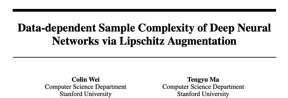
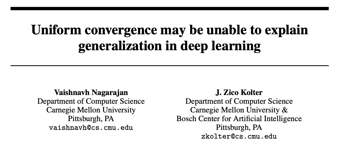
Theorem$^\star$ (Nagarajan et. al. (2019), Wei et. al (2020), etc.)

\begin{align*} \mathrm{TestError}_0( { h}) &\leq \mathrm{TrainingError}_{\gamma}( { h}) + \tilde{\mathcal{O}}\left( \frac{ \kappa_{\rm Jacobian}(h, S) %\mathrm{KL}\left(\mathcal{N}({ h}, \sigma^2) || \mathcal{P}\right) } {\gamma \; \sqrt{m}} \right) \end{align*}

$^\star$ Simplified informal statement of results.

\kappa_{\rm Jacobian}(h, S) \propto

\Big \{

\mathrm{L}_{\mathrm{jacobian}}(h,x_i)

\max_{(x_i,y_i) \in S}

Generalization via Jacobian Sensitivity

With high probability over the training data S, for any $ h \in \mathcal{H} $

\kappa_{\rm Jacobian}(h, S) \propto \max_{(x_i,y_i) \in S} \Big\{ \mathsf{L}_{\mathrm{Jacobian}}(h, x_i) \;,\; \frac{1}{\mathrm{r}_{\mathrm{Jacobian}}(h, x_i)} \Big \}

\mathrm{L}_{\mathrm{jacobian}}(h,x_i) %\| \nabla h(x_i) \|_2\|\nabla h(x)\|_2 \ll { \mathrm{L}_{\mathrm{global}}}(h) %\approx 0 %, \quad r_{\mathrm{jacobian}}}(h, x_i) \approx 0 %\forall\; x, \tilde{x} \in \mathcal{X}\quad \| h(\tilde{x}) - h(x) \|_2 \leq {\color{red} \mathrm{L}_{\mathrm{global}}}(h) \|\tilde{x} - x \|_{2}

For some $ (x_i, y_i) $,

Theorem$^\star$ (Nagarajan et. al. (2019), Wei et. al (2020), etc.)

\ll \frac{1}{{ \mathrm{r}_{\mathrm{Jacobian}}}(h, x_i)}

When the local linear approximation is fragile
e.g. high curvature,
non-linearity, etc.

$^\star$ Simplified informal statement of results.

Sensitivity$(h)$

Bound on

$\mathrm{TestError}_0(h)$

Bartlett et. al. (2017),

Neyshabur et. al (2017), etc.

Nagarajan et. al. (2019),

Wei et. al (2020), etc.

Global

Jacobian

$1$

$0$

Best of both worlds?

Sensitivity-based capacity

Is there a rigorous generalization bounds based on intermediate sensitivity?

Local Sensitivity Oracles

\mathrm{dist}(\hat{h}, h) \leq

A local sensitivity oracle$^{\star}$ provides a radius $\mathrm{r}_{\mathrm{local}}$ such that,

Model

Input

Desired Sensitivity Level

\mathrm{r}_{\mathrm{local}}

\implies \| \hat{h}(x) - h(x) \|_2 \leq \mathsf{L} \;\mathrm{dist}(\hat{h}, h)

(h, x, \mathsf{L})

$^\star$ An oracle is a black box assumed to answer queries, without revealing how.

We assume that the local sensitivity oracle is stable:

\| r_{\rm local}(\hat{h}, x, \mathsf{L}) - r_{\rm local}(h, x, \mathsf{L}) \|_2 \leq \mathrm{dist}(\hat{h}, h)

Local radius within $h$ exhibits desired sensitivity at $x$

The desired level of local sensitivity $\mathsf{L}$

Generalization via Local Sensitivity

$^\star$ Simplified informal statement of results.

$\gamma, \mathsf{L}$ are hyper-parameters chosen before observing data

\begin{align*} \mathrm{TestError}_0( { h}) &\leq \mathrm{TrainingError}_{\gamma}( { h}) + \tilde{\mathcal{O}}\left( \frac{ \kappa_{\rm local}(h, S, \mathsf{L}) %\mathrm{KL}\left(\mathcal{N}({ h}, \sigma^2) || \mathcal{P}\right) } {\gamma \; \sqrt{m}} \right) \end{align*}

With high probability over the training data S, for any $ h \in \mathcal{H} $

\kappa_{\rm local}(h, S, \mathsf{L}) \propto \max_{(x,y) \in S} \Big\{ \mathsf{L} \;,\; \frac{1}{\mathrm{r}_{\mathrm{local}}(h, x, \mathsf{L})} \Big \}

Theorem$^\star$ (Stable Local Sensitive Oracle)

With high probability over the training data S, for any $ h \in \mathcal{H} $

\kappa_{\rm local}(h, S, \mathsf{L}) \propto \max_{(x,y) \in S} \Big\{ \mathsf{L} \;,\; \frac{1}{\mathrm{r}_{\mathrm{local}}(h, x, \mathsf{L})} \Big \}

Generalization via Local Sensitivity

$^\star$ Simplified informal statement of results.

$\gamma, \mathsf{L}$ are hyper-parameters chosen before observing data

Intermediate sensitivity can provide rigorous generalization bounds for all hypothesis classes!

Search for the optimal sensitivity level $\mathsf{L}$
for each model $h$ and training data $S$

Theorem$^\star$ (Stable Local Sensitive Oracle)

Takeaways

Any intermediate sensitivity level corresponds to a generalization bound.
Optimal choice is data and model-dependent.
In general, local sensitivity oracles can be hard to compute exactly or approximately$^\star$

$^\star$ Exact computation is NP-hard even for shallow feedforward neural networks as per (Scaman et. al. 2016)

Evaluate Rigorously

Identify Parsimony

Roadmap

Measure Locally

Structure in the interactions between the model and data

aka Occam's razor
Start simple, add complexity only if essential.

Identify Parsimony

\| \hat{h}(x) - h(x) \|_2 \leq \mathsf{L} \;\mathrm{dist}(\hat{h}, h)

What does it mean for a model $h$
to exhibit low or high sensitivity?

Interpretation$^{\star}$ of sensitivity depends
on the scale of the original output: $\|h(x)\|_2$

Scale and Sensitivity

$^\star$ A salary increase of $1000 is insignificant to Jeff Bezos but significant to me.

\| \hat{h}(x) - h(x) \|_2 \leq \mathsf{L} \;\mathrm{dist}(\hat{h}, h)

Misleading for a particular $h$ and input $x$ when the scale varies significantly

worst-case scale across $\mathcal{H}$ and $\mathcal{X}$

Local sensitivity should be
proportional to the local scale:
$\sup_{\hat{h}\; \mathrm{ nearby }\; h}\; \sup_{\tilde{x}\; \mathrm{ nearby }\; {x}} \|\hat{h}(\tilde{x})\|_2$.

Scale and Sensitivity

\mathsf{L}_{\rm global} \propto \sup_{h \in \mathcal{H}} \;\sup_{x \in \mathcal{X}} \; \|h(x)\|_2

Roots of Local Sensitivity

My brain in full

Reading

The Local Parsimony Principle
Locally, complex models $\approx$ simpler models

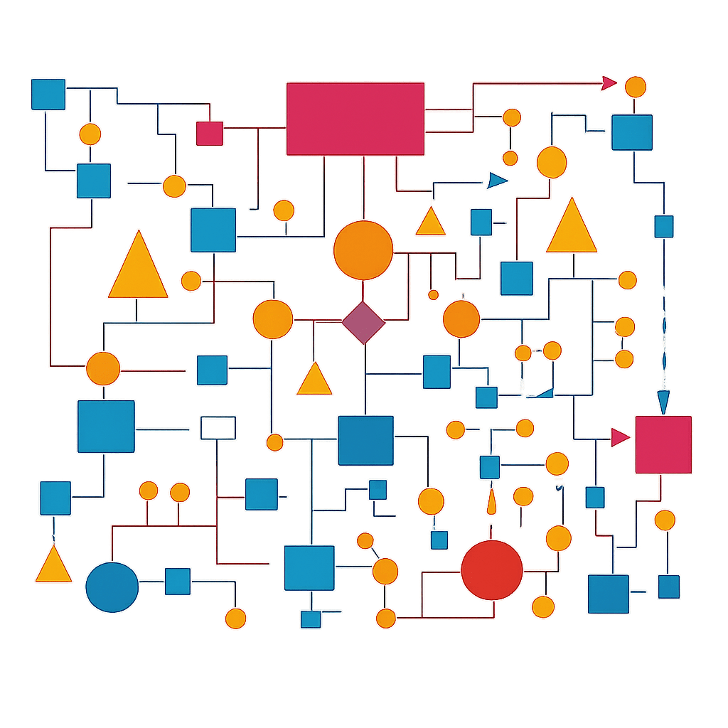
Different simpler models of varying complexity for each $ (h, x) $

Listening

Thinking

Local sensitivity should be
proportional to the local scale:
$\sup_{\hat{h}\; \mathrm{ nearby }\; h}\; \sup_{\tilde{x}\; \mathrm{ nearby }\; {x}} \|\hat{h}(\tilde{x})\|_2$.

Local Parsimony in Deep Learning

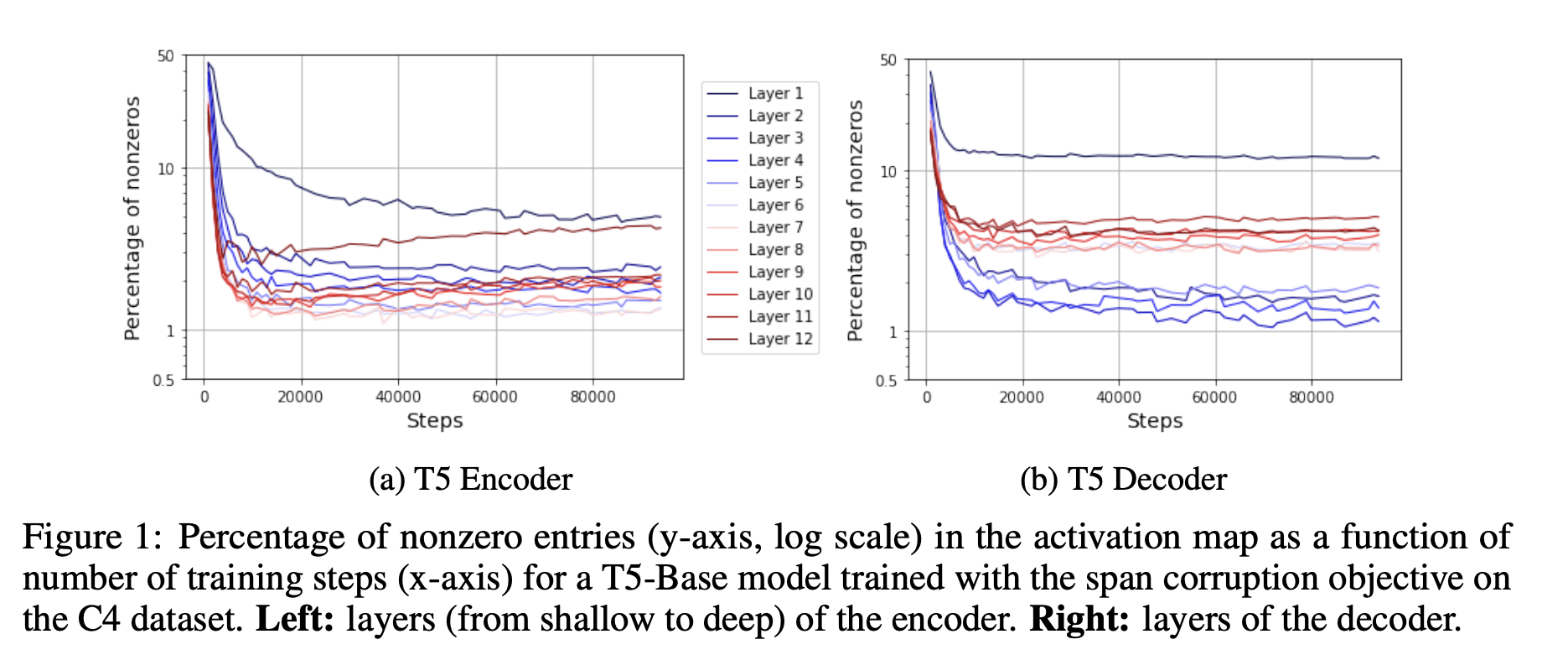
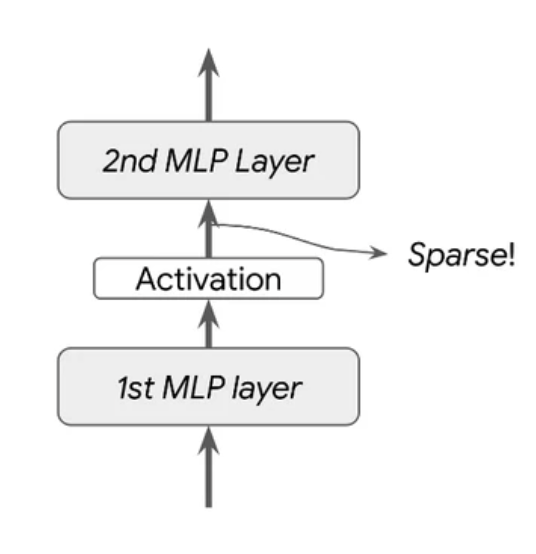
Only 3% of neurons are needed at any input.

Neural networks are not brains but do exhibit local parsimony

Local Parsimony in Deep Learning

We will now show a systematic framework
linking parsimony and sensitivity.

Each step uses the example of a feedforward map

h(x) = \texttt{ReLU}(W x)

Observe Parsimony

Observe parsimony in the interaction between model and data

The output $h(x) $ is sparse with an index set J of size $s$ containing only zero entries

$ s$

$\Big($

$\Big)$

= $\texttt{ReLU}$

$x$

$W$

$h(x)$

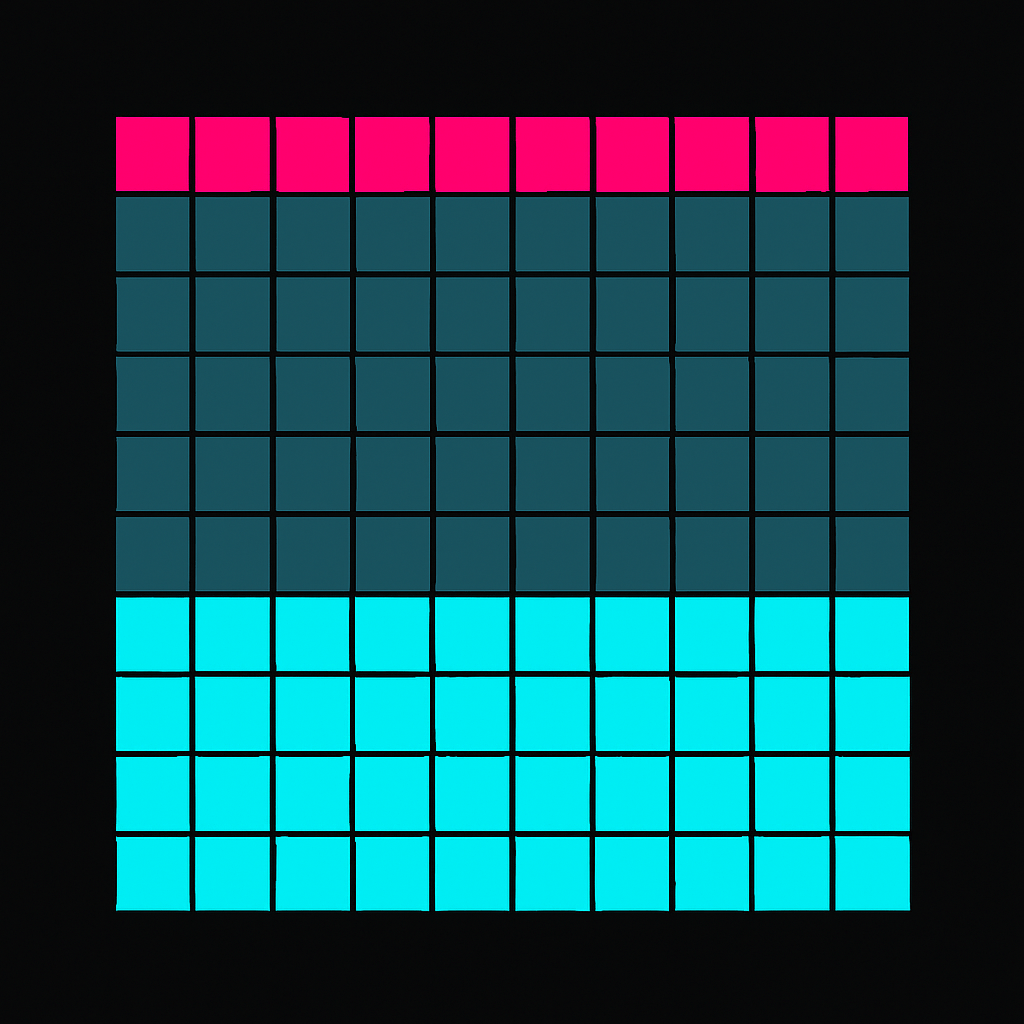
${J} $

${J^c} $

An observation has 3 parts

Form

Degree

Context

(sparsity, $s$, $ J$)

Identify and Isolate

Identify the active and inactive parts

$W[J,:]$ is active and $W[J^c,:]$ is inactive

$ s$

${J^c} $

$\Big($

$\Big)$

= $\texttt{ReLU}$

$x$

$W$

$h(x)$

${J} $

Isolate the structural trigger of parsimony

W[i] x \leq 0 \implies h(x) [i] = 0

Reduce and Localize

Reduce the complexity of the model at an input

$ s$

${J} $

$\Big($

$\Big)$

= $\texttt{ReLU}$

$x$

$W$

$h(x)$

${J} $

$\Big($

$\Big)$

= $\texttt{ReLU}$

$x$

$h_{J}(x)$

${J^c} $

${J^c} $

$\mathcal{P}_{J,:} (W)$

$\mathcal{P}_{J,:} (W)$ = rows of $W$ in $J^c$ are zeroed

Reduce the complexity of the model at an input

${J} $

$\Big($

$\Big)$

= $\texttt{ReLU}$

$x$

$\mathcal{P}_{J,:} (W)$

$h_{J}(x)$

${J^c} $

At $x$, the complex model $h$ is equivalent to the simpler model $h_{J}$

$\|h(x)\|_2 = \|h_J(x)\|_2 \leq \|\mathcal{P}_{J,:}(W)\|_2 \|x\|_2$

$ s$

${J} $

$h(x)$

${J^c} $

= $\texttt{ReLU}$

Reduce and Localize

Localize the reduction in complexity to nearby$^\star$ models

\mathrm{dist}(\hat{h}, h) \leq r_{\rm sparse}(h,x, J) \implies \hat{h}(x) = \hat{h}_J(x)

${J} $

$\Big($

$\Big)$

= $\texttt{ReLU}$

$x$

$\hat{h}_{J}(x)$

${J^c} $

Local radius

\mathrm{r}_{\rm sparse} ( h, x, J) = \frac{ \max \Big\{\; \mathcal{P}_{J^c,:}(W) x \;,\; 0\;\Big\} %\mathrm{ReLU}\left(\texttt{sort}(- W x, s)\right) }{\| \mathcal{P}_{J^c,:}(W)\|_{2,\infty} \; \|x\|_2}

$\mathcal{P}_{J,:} (\hat{W})$

Reduce and Localize

$^\star$ For an appropriately chosen distance metric

Measure Sensitivity

Measure sensitivity locally within the neighborhood

Local radius

\begin{align*} \|\hat{h}(x) - h(x)\|_2 &= \|\hat{h}_J(x) - h_J(x)\|_2 \\ &\leq \mathsf{L}_{\rm sparse} ( h, x, J) \;\mathrm{dist}(\hat{h}, h) \end{align*}

For nearby models $\hat{h}$ within the local radius,

Local sensitivity

\mathsf{L}_{\rm sparse} ( h, x, J) = \| \mathcal{P}_{J,:}(W)\|_2 \|x\|_2

Local sensitivity is proportional to the local scale

Measure local sensitivity

Measure sensitivity locally within the neighborhood

$\mathsf{L}_{\rm jacobian}(h,x) \leq \mathsf{L}_{\rm sparse} (h,x, J) \leq \mathsf{L}_{\rm global}$

For all observations of parsimony with context $J$

$\mathsf{r}_{\rm jacobian}(h,x) \leq \mathsf{r}_{\rm sparse} (h, x, J) \leq \mathrm{r}_{\rm global} = \infty$

A larger local sensitivity holding within a larger neighborhood

Local radius

Local sensitivity

\mathsf{L}_{\rm sparse} ( h, x, J) = \| \mathcal{P}_{J,:}(W)\|_2 \|x\|_2

Collect and Aggregate

So far, we saw how a single observation of parsimony yields a local measure of sensitivity.

\mathsf{L}_{\rm sparse} ( h, x, s) = \max_{J: |J|=s} \mathsf{L}_{\rm sparse} ( h, x, J)

\mathrm{r}_{\rm sparse} ( h, x, s) = \max_{J: |J|=s} \mathrm{r}_{\rm sparse} ( h, x, J)

Collect and aggregate measurements across different contexts for a fixed degree of sparsity $s$

Vary $s$ to interpolate between Jacobian and global sensitivity

Chain Sequentially

\mathsf{L}_{\rm sparse} (h_{\rm single}, x, s_1)

\rightarrow \; \mathrm{r}_{\rm sparse} ( h_{\rm multi}, x, \vec{s})

${J}_1 $

${J}^c_1 $

${J}_1 $

${J}^c_1 $

${J}_2 $

${J}^c_3 $

$W_1$

$W_2$

$W_3$

${J}^c_2 $

${J}_2 $

${J}_3 $

${J}^c_2 $

\mathrm{r}_{\rm sparse} ( h_{\rm single}, x, s_1)

\rightarrow \; \mathsf{L}_{\rm sparse} ( h_{\rm multi}, x, \vec{s})

From single layer feedforward map to multiple layers

\texttt{ReLU}(W x)

h_{\rm single}(x)

\rightarrow \; h_{\rm multi}(x) = h_{K+1} \circ h_{K} \cdots \circ h_1 (x)

\rightarrow W_{K+1} \texttt{ReLU}\Big(W_K \texttt{ReLU}(W_{K-1} \cdots \texttt{ReLU}(W_1 x) \cdot ) \Big)

$\vec{s} = (s_1, s_2, \ldots, s_K)$

A Sparse Local Sensitivity Recap

This workflow can be reproduced for other $\mathcal{H}$
e.g convolutional networks, transformers,
dictionary learning, center-based clustering etc.

Observe Parsimony

Collect
and Aggregate

Identify
and Isolate

Measure
Sensitivity

Reduce
and Localize

Chain
Sequentially

Evaluate Rigorously

Identify Parsimony

Measure Locally

Sparsity-aware Generalization Theory

Radius within $h$ exhibits desired stable sparsity at $x$

The sensitivity corresponding to the desired level of stable sparsity $\mathsf{L}$

Trade-off margin-threshold $\gamma$ and sparsity levels $\vec{s}$ for an optimal bound for each model $h$ and data $S$!

Theorem (Sparse local sensitivity-normalized margin bounds$^\star$)

\begin{align*} \mathrm{TestError}_0( { h}) &\leq \mathrm{TrainingError}_{\gamma}(h) + \tilde{\mathcal{O}}\left( \sqrt{ \frac{ \kappa_{\rm sparse}(h, S, \vec{s}) %\mathrm{KL}\left(\mathcal{N}({ h}, \sigma^2) || \mathcal{P}\right) } {\gamma \; m}} \right) \end{align*}

With high probability over the training data S, for any $ h \in \mathcal{H} $

\kappa_{\rm sparse}(h, S, \vec{s}) \coloneqq \max_{(x,y) \in S} \Big\{ \mathsf{L}(\vec{s}) \;,\; \frac{1}{\mathrm{r}_{\mathrm{sparse}}(h, x, \mathsf{L}(\vec{s}))} \Big \}

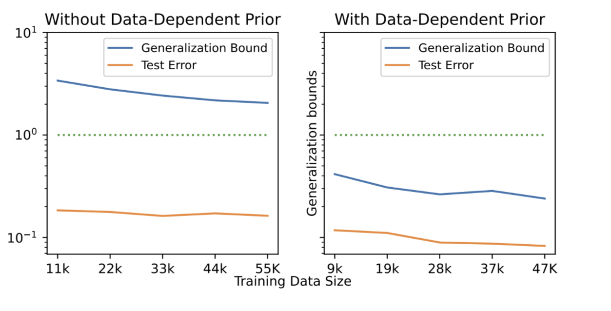
Experimental Evaluation

Random Initialization

Pretrained Initialization

Optimized generalization bound for overparameterized
3-layer feedforward networks on MNIST

11k

22k

33k

44k

55k

11k

22k

33k

44k

55k

0.1

Size of Training Data

Effective Dimensionality Ratio

\tau(x,\gamma) := \frac{\# \mathrm{params}(h_{\mathrm{simple},x})}{\#\mathrm{params}(h)} \; \in [0,1]

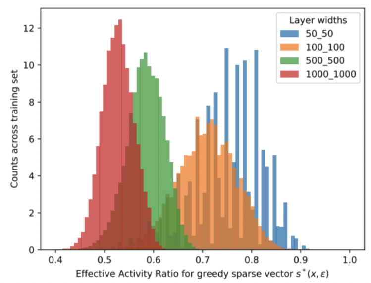
Histogram of $ \tau(h, x, \gamma) $ across training data

0.4

0.5

0.6

0.7

0.8

0.9

1.0

Models with larger layer widths have
smaller effective dimensionality ratio

Conclusion

Results for general hypothesis classes $ \mathcal{H} $
using a local sensitivity oracle

Systematic framework shown via feedforward neural networks
Applicable to other forms of parsimony (e.g. rank)

Identify Parsimony, Measure Locally, Evaluate Rigorously

A theory of generalization via local parsimony

Evaluate Rigorously

Identify Parsimony

Roadmap

Measure Locally

Evaluate Rigorously

Classification Task

Classification Task

Classification Task

Classification Task

Supervised Learning

Generalization

Classification Task

Classification Task

Classification Task

Generalization

Classification Task

Generalization

Classification Task

Generalization Bounds

Generalization Bounds

Generalization Bounds

Capacity measures in Deep Learning

Sensitivity-based capacity

Generalization via Global Sensitivity

Evaluate Rigorously

Identify Parsimony

Roadmap

Measure Locally

Measure Locally

Generalization via Jacobian Sensitivity

Generalization via Jacobian Sensitivity

Sensitivity-based capacity

Local Sensitivity Oracles

Generalization via Local Sensitivity

Generalization via Local Sensitivity

Takeaways

Evaluate Rigorously

Identify Parsimony

Roadmap

Measure Locally

Identify Parsimony

Scale and Sensitivity

Scale and Sensitivity

Roots of Local Sensitivity

Local Parsimony in Deep Learning

Local Parsimony in Deep Learning

Observe Parsimony

Identify and Isolate

Reduce and Localize

Reduce and Localize

Reduce and Localize

Measure Sensitivity

Measure local sensitivity

Collect and Aggregate

Chain Sequentially

A Sparse Local Sensitivity Recap

Evaluate Rigorously

Identify Parsimony

Measure Locally

Sparsity-aware Generalization Theory

Experimental Evaluation

Effective Dimensionality Ratio

Conclusion

Intermediate sensitivity \( \rightarrow \) Generalization bounds

Local parsimony \(\rightarrow \) Intermediate sensitivity

Thank you!

ML Theory Reading Group meeting

More from Ramchandran Muthukumar

A theory of generalization
via local parsimony