
Ranveer Aggarwal
Software Engineer
Bruce Walter, Pramook Khungurn, Kavita Bala
A presentation by:
Ranveer Aggarwal &
Abhinav Gupta
Guide: Prof. Parag Chaudhuri
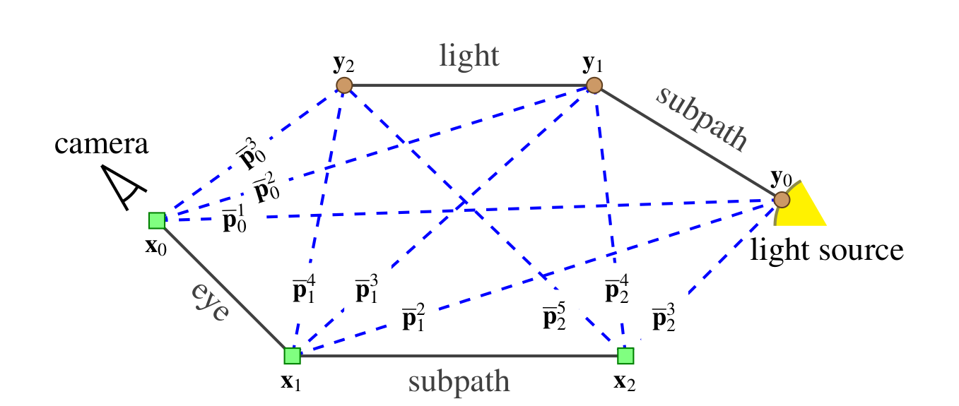
Virtual Point Lights: Recursively trace a direction from light source. Generate VPL at every hit with reducing intensity.
Virtual Sensor Points: Similar to VPL. Start from the eye and generate VPS at every hit.
1. Energy Conservation and Favoring Shorter Eye Paths
2. Clamping
3. Diffuse VPLs
4. Exclusion of High-Variance Eye Subpaths
Computing illumination from tens of thousands of lights is expensive.
Solution: Clustering!
Cluster similar lights together and treat them as a single light.
Give theoretical upper bound on error.
Choose cut with error less than a perceptibility threshold (Weber’s Law).
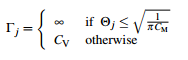
A set of nodes such that exactly one node from the set is present in any path from the root to a leaf.
Set the lightcut to { root }.
Computer the error bound for the light cut. If this is less that the threshold we are done.
Pick the node with the maximum error and refine it by replacing it with it’s children in the lightcut.
Go to Step 2
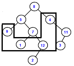
Use a bottom-up greedy strategy.
Pair lights/clusters with the highest similarity.
Similarity Metric is based on the diagonal length of the bounding box and the cone-angle of the direction (in case of oriented lights)
Representative light is randomly chosen with probabilities in proportion to intensities.
Have to evaluate Lots of VPLs and VPSs. Building a light graph for is expensive.
Build an implicit graph from individual light trees.
Traverse the light graph by refining a node in one of the trees.
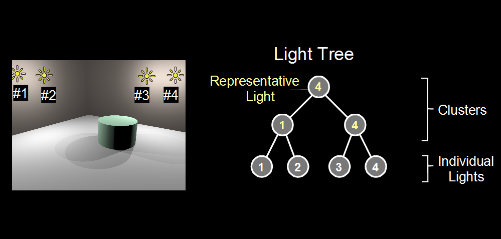
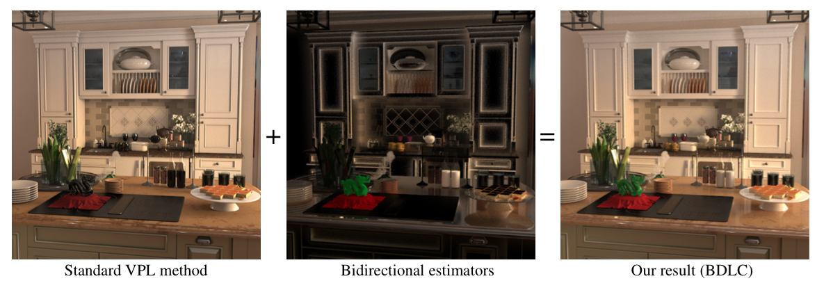
* The above result has been taken from the original paper and not rendered by us.
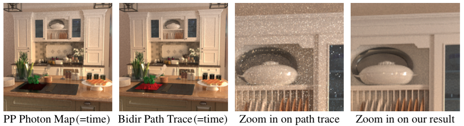
* The above result has been taken from the original paper and not rendered by us.
Bruce Walter, Pramook Khungurn, and Kavita Bala. Bidirectional lightcuts. ACM Trans. Graph., 31(4):59:1–59:11, July 2012.
Bruce Walter, Adam Arbree, Kavita Bala, and Donald P. Greenberg. Multidimensional lightcuts. ACM Trans. Graph., 25(3):1081–1088, July 2006.
Bruce Walter, Sebastian Fernandez, Adam Arbree, Kavita Bala, Michael Donikian, and Donald P. Greenberg. Lightcuts: A scalable approach to illumination. ACM Trans. Graph., 24(3):1098–1107, July 2005.
By Ranveer Aggarwal


