Modelling hydrogen in materials:
component to reactor scale
\frac{\partial c_\mathrm{m}}{\partial t} = \nabla \cdot \left(D\nabla c_\mathrm{m} \right) + S - \sum \frac{\partial c_\mathrm{t,i}}{\partial t}
\frac{\partial c_\mathrm{t, i}}{\partial t} = k_i \ c_\mathrm{m} \ (n_\mathrm{trap,i} - c_\mathrm{t,i}) - p_i c_\mathrm{t,i}
Reminder: McNabb & Foster model
Let's solve the system analytically
\frac{\partial c_\mathrm{m}}{\partial t} = \nabla \cdot \left(D\nabla c_\mathrm{m} \right) + S - \sum \frac{\partial c_\mathrm{t,i}}{\partial t}
\frac{\partial c_\mathrm{t, i}}{\partial t} = k_i \ c_\mathrm{m} \ (n_\mathrm{trap,i} - c_\mathrm{t,i}) - p_i c_\mathrm{t,i}
Let's solve the system analytically
Simplification #1: 1D domain \(L\)
\frac{\partial c_\mathrm{m}}{\partial t} = \frac{\partial}{\partial x} \left(D \frac{\partial}{\partial x} c_\mathrm{m} \right) + S - \sum \frac{\partial c_\mathrm{t,i}}{\partial t}
\frac{\partial c_\mathrm{t, i}}{\partial t} = k_i \ c_\mathrm{m} \ (n_\mathrm{trap,i} - c_\mathrm{t,i}) - p_i c_\mathrm{t,i}
Let's solve the system analytically
Simplification #1: 1D domain \(L\)
Simplification #2: 1 material
\frac{\partial c_\mathrm{m}}{\partial t} = \frac{\partial}{\partial x} \left(D \frac{\partial}{\partial x} c_\mathrm{m} \right) + S - \sum \frac{\partial c_\mathrm{t,i}}{\partial t}
\frac{\partial c_\mathrm{t, i}}{\partial t} = k_i \ c_\mathrm{m} \ (n_\mathrm{trap,i} - c_\mathrm{t,i}) - p_i c_\mathrm{t,i}
Let's solve the system analytically
D, S, k, p, n = \mathrm{constants}
Simplification #1: 1D domain \(L=1\)
Simplification #2: 1 material
Simplification #3:
\frac{\partial c_\mathrm{m}}{\partial t} = D \frac{\partial^2 c_\mathrm{m}}{\partial x^2} + S - \sum \frac{\partial c_\mathrm{t,i}}{\partial t}
\frac{\partial c_\mathrm{t, i}}{\partial t} = k_\mathrm{i} \ c_\mathrm{m} \ (n_\mathrm{trap,i} - c_\mathrm{t,i}) - p_\mathrm{i} c_\mathrm{t,i}
Let's solve the system analytically
D, S, k, p, n = \mathrm{constants}
Simplification #1: 1D domain \(L\)
Simplification #2: 1 material
Simplification #3:
Simplification #4: Steady state
0 = k_\mathrm{i} \ c_\mathrm{m} \ (n_\mathrm{trap,i} - c_\mathrm{t,i}) - p_\mathrm{i} c_\mathrm{t,i}
0 = D \frac{\partial^2 c_\mathrm{m}}{\partial x^2} + S
💡At steady state, the mobile concentration is independent of trapping
Let's solve the system analytically
0 = k_\mathrm{i} \ c_\mathrm{m} \ (n_\mathrm{trap,i} - c_\mathrm{t,i}) - p_\mathrm{i} c_\mathrm{t,i}
0 = D \frac{\partial^2 c_\mathrm{m}}{\partial x^2} + S
c_\mathrm{t,i} = \frac{n_\mathrm{trap,i}}{1+ \frac{p_\mathrm{i}}{k_\mathrm{i} \ c_\mathrm{m}}}
Oriani's model
Let's solve the system analytically
0 = D \frac{\partial^2 c_\mathrm{m}}{\partial x^2} + S
c_\mathrm{t,i} = \frac{n_\mathrm{trap,i}}{1+ \frac{p_\mathrm{i}}{k_\mathrm{i} \ c_\mathrm{m}}}
\frac{\partial^2 c_\mathrm{m}}{\partial x^2} = \frac{-S}{D}
\frac{\partial c_\mathrm{m}}{\partial x} = \frac{-S}{D} x + K_1
c_\mathrm{m} = \frac{-S}{2\ D} x^2 + K_1 \ x + K_2
2 unknowns =
2 equations =
2 boundary conditions
Let's solve the system analytically
c_\mathrm{t,i} = \frac{n_\mathrm{trap,i}}{1+ \frac{p_\mathrm{i}}{k_\mathrm{i} \ c_\mathrm{m}}}
c_\mathrm{m} = \frac{-S}{2\ D} x^2 + K_1 \ x + K_2
c_\mathrm{m}(x=0) = 1 \\
c_\mathrm{m}(x=1) = 0
Let's solve the system analytically
c_\mathrm{t,i} = \frac{n_\mathrm{trap,i}}{1+ \frac{p_\mathrm{i}}{k_\mathrm{i} \ c_\mathrm{m}}}
c_\mathrm{m} = \frac{-S}{2\ D} x^2 + K_1 \ x + K_2
K_2 = 1 \\
\frac{-S}{2\ D} + K_1 + K_2 = 0
K_2 = 1 \\
K_1= \frac{-S}{2\ D} - 1
Let's solve the system analytically
c_\mathrm{t,i} = \frac{n_\mathrm{trap,i}}{1+ \frac{p_\mathrm{i}}{k_\mathrm{i} \ c_\mathrm{m}}}
c_\mathrm{m} = \frac{-S}{2\ D} x^2 - (\frac{S}{2\ D} + 1) \ x + 1

- Steady state
- 1 material
- Homogeneous temperature
- 1D
We can solve it numerically
Component modelling
Experimental analysis
3 main numerical methods
Finite Difference Method (FDM)
Finite Element Method (FEM)
Finite Volume Method (FVM)
Let's not bother
\frac{\partial c }{\partial x} \approx \frac{c(x=x_{i+1}) - c(x=x_{i})}{x_{i+1} - x_{i}}

3 main numerical methods
\frac{\partial c }{\partial x} \approx \frac{c(x=x_{i+1}) - c(x=x_{i})}{x_{i+1} - x_{i}}
2
Finite Difference Method (FDM)
Finite Element Method (FEM)
Different ways of discretising space
3 main numerical methods
Finite Difference Method (FDM)
Finite Element Method (FEM)
2
✅Easy to implement in 1D
❌Hard to extend to 2D/3D
✅Better performances for hyperbolic problems
✅Can be applied to complex geometries
✅Better performances for parabolic problems
❌Complex implementation from scratch
We don't care
There are a handful of H transport codes
TMAP7
TMAP8
MHIMS
FESTIM
COMSOL
Abaqus
There are a handful of H transport codes
TMAP7
TMAP8
MHIMS
FESTIM
COMSOL
Abaqus
1D
1D/2D/3D
TESSIM
There are a handful of H transport codes
TMAP7
MHIMS
FDM
FEM
TESSIM
TMAP8
FESTIM
COMSOL
Abaqus
There are a handful of H transport codes
TMAP7
TMAP8
MHIMS
FESTIM
COMSOL
Abaqus
Proprietary
Open-source
Closed-source
TESSIM
COMSOL
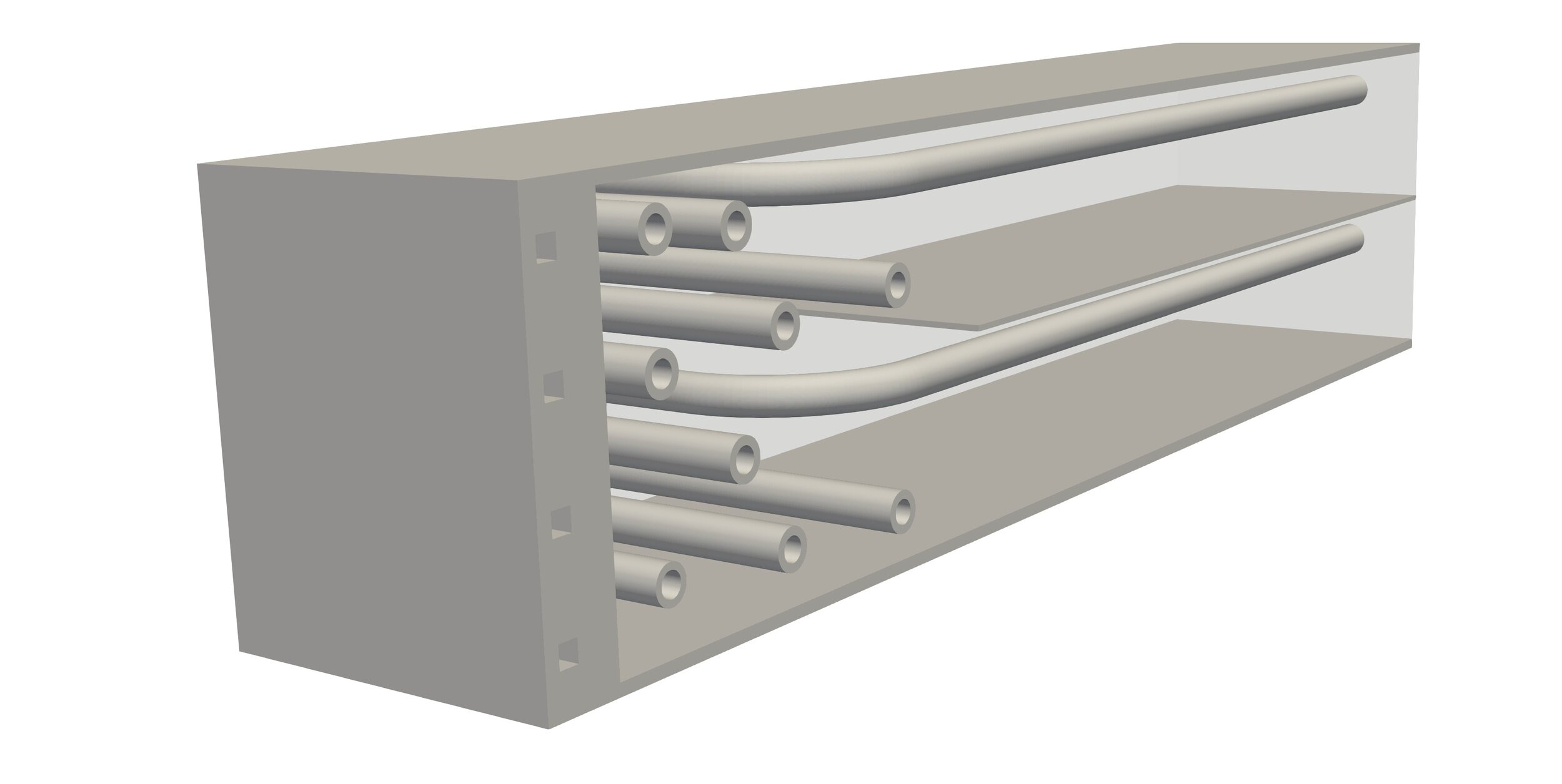
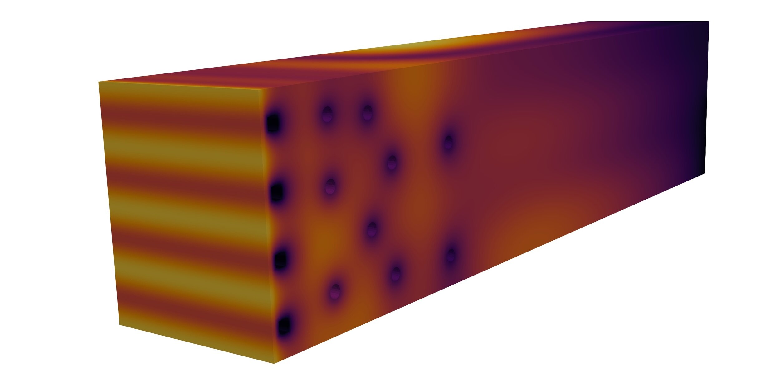
- ARC's breeding blanket
- Source of tritium from neutronics calculations
- Heat transfer + Fluid dynamics + H transport
- Steady state
- Computation time 8h
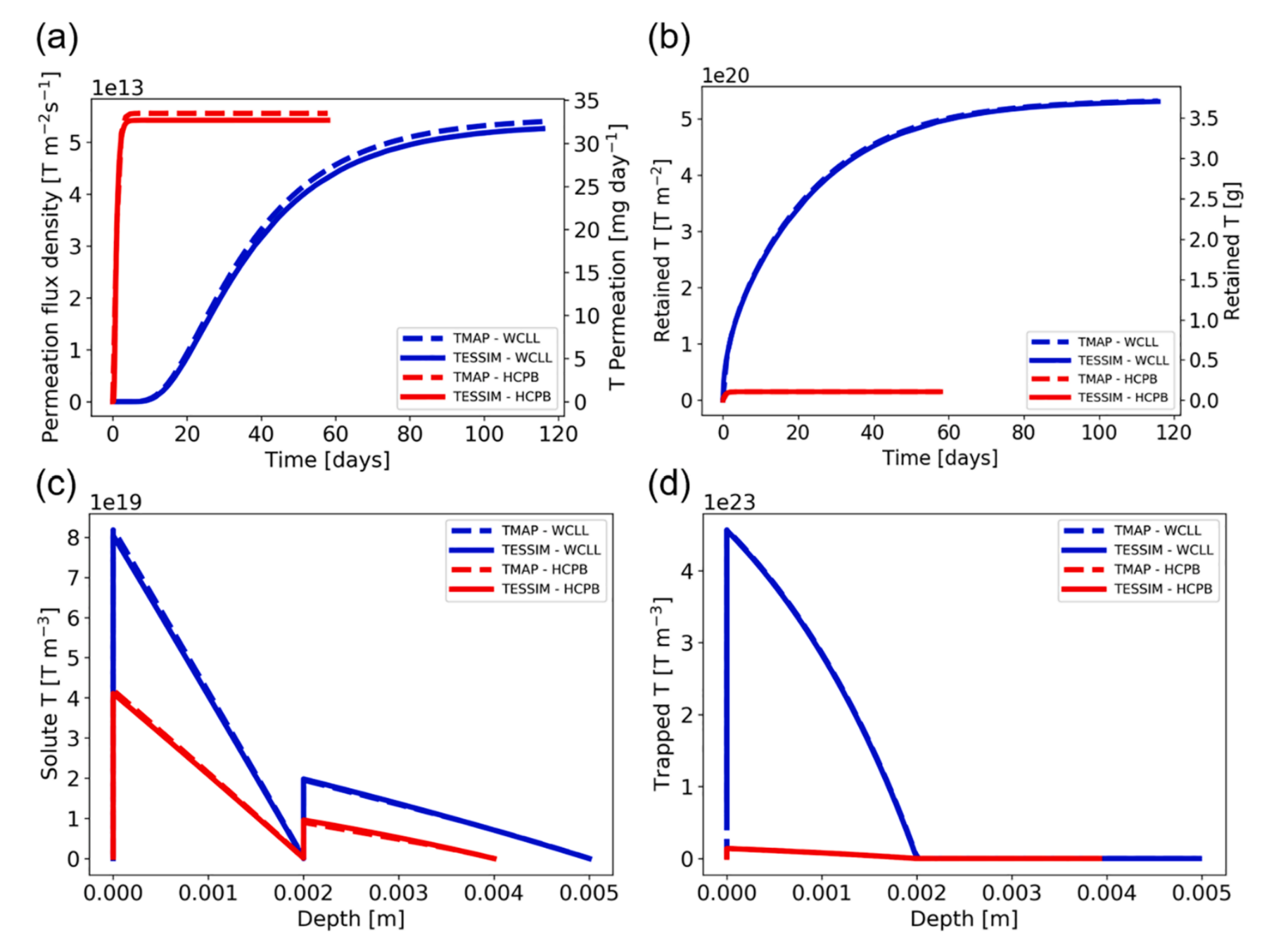
TMAP7 and TESSIM
- W on Eurofer
- 1D
- Agreement between TMAP and TESSIM
FESTIM
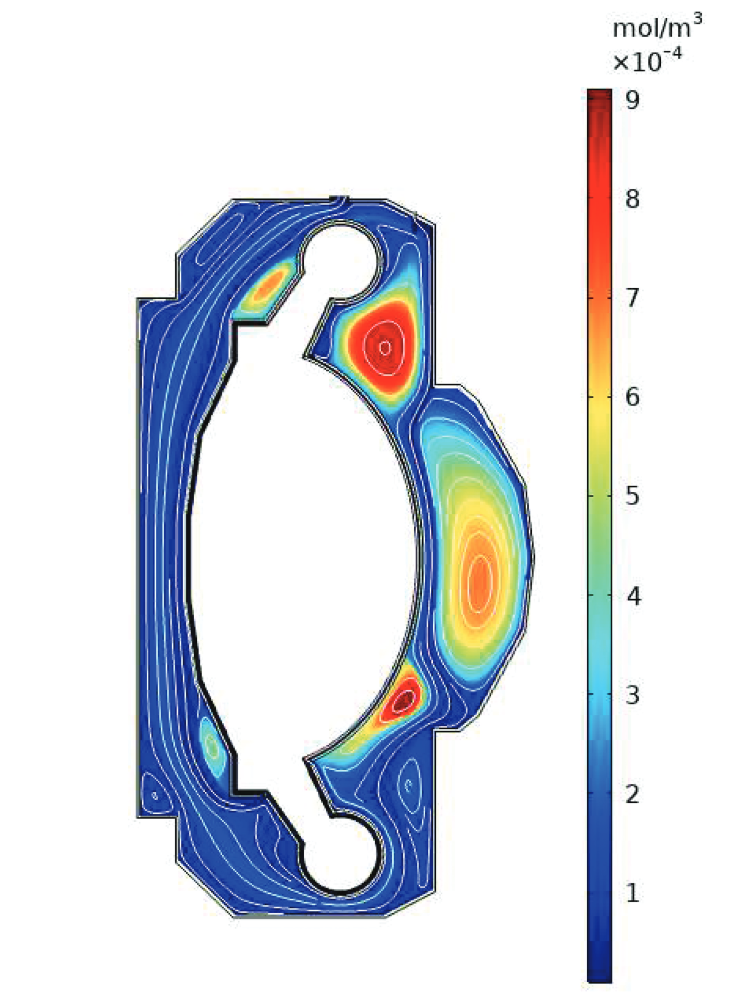
Simulation of a WCLL breeding blanket from CAD files
1) Mesh generation
2) Heat transfer simulation
3) 2D slice
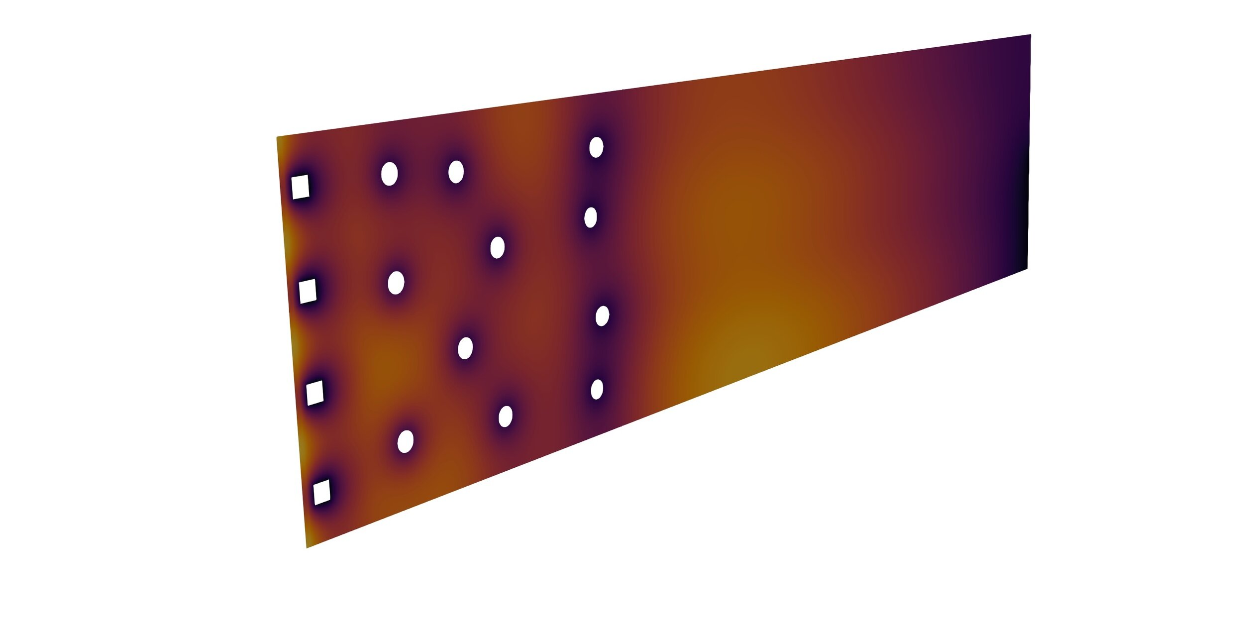
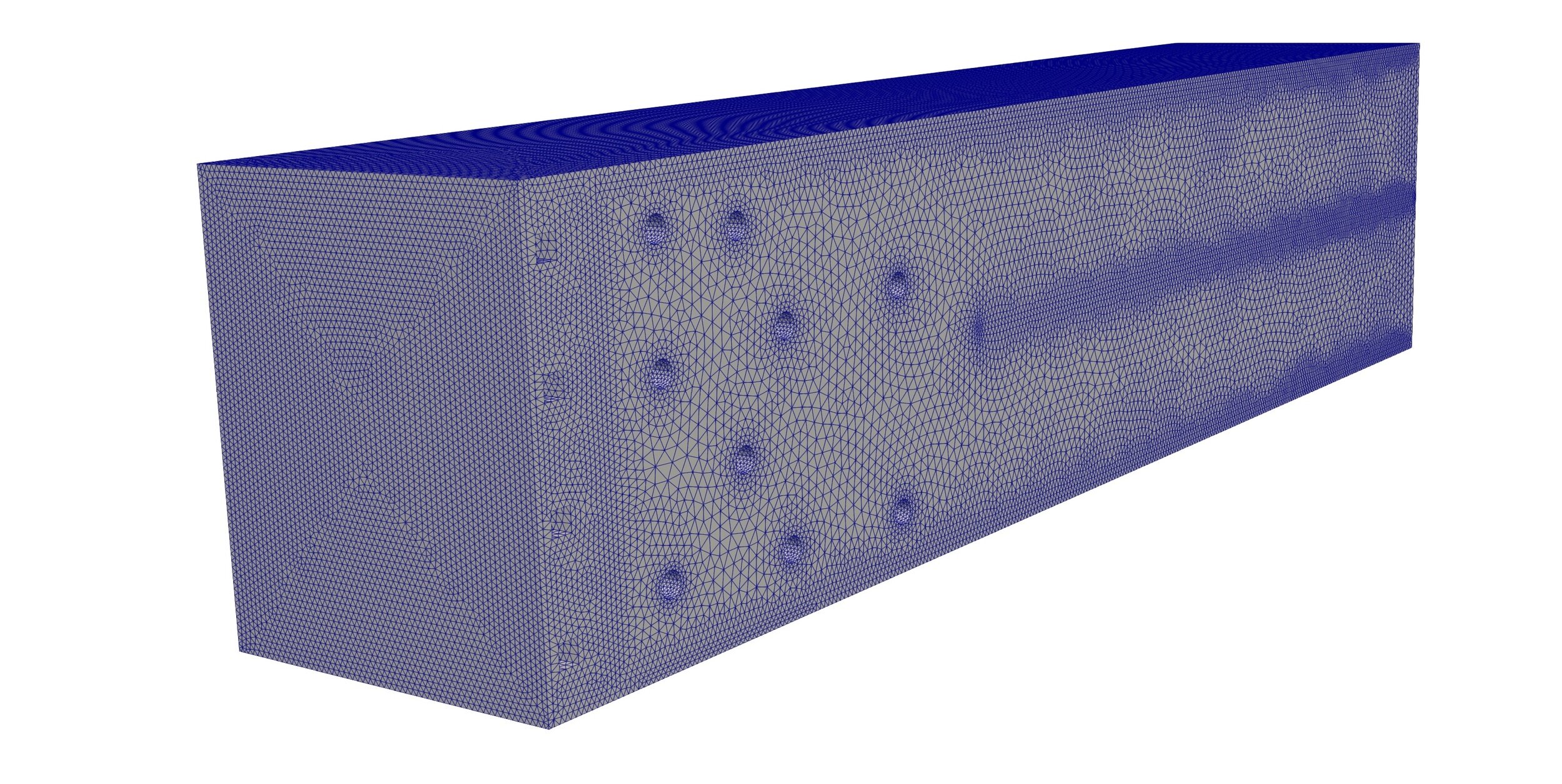
FESTIM
Simulation of a WCLL breeding blanket from CAD files
1) Mesh generation
2) Heat transfer simulation
3) 2D slice
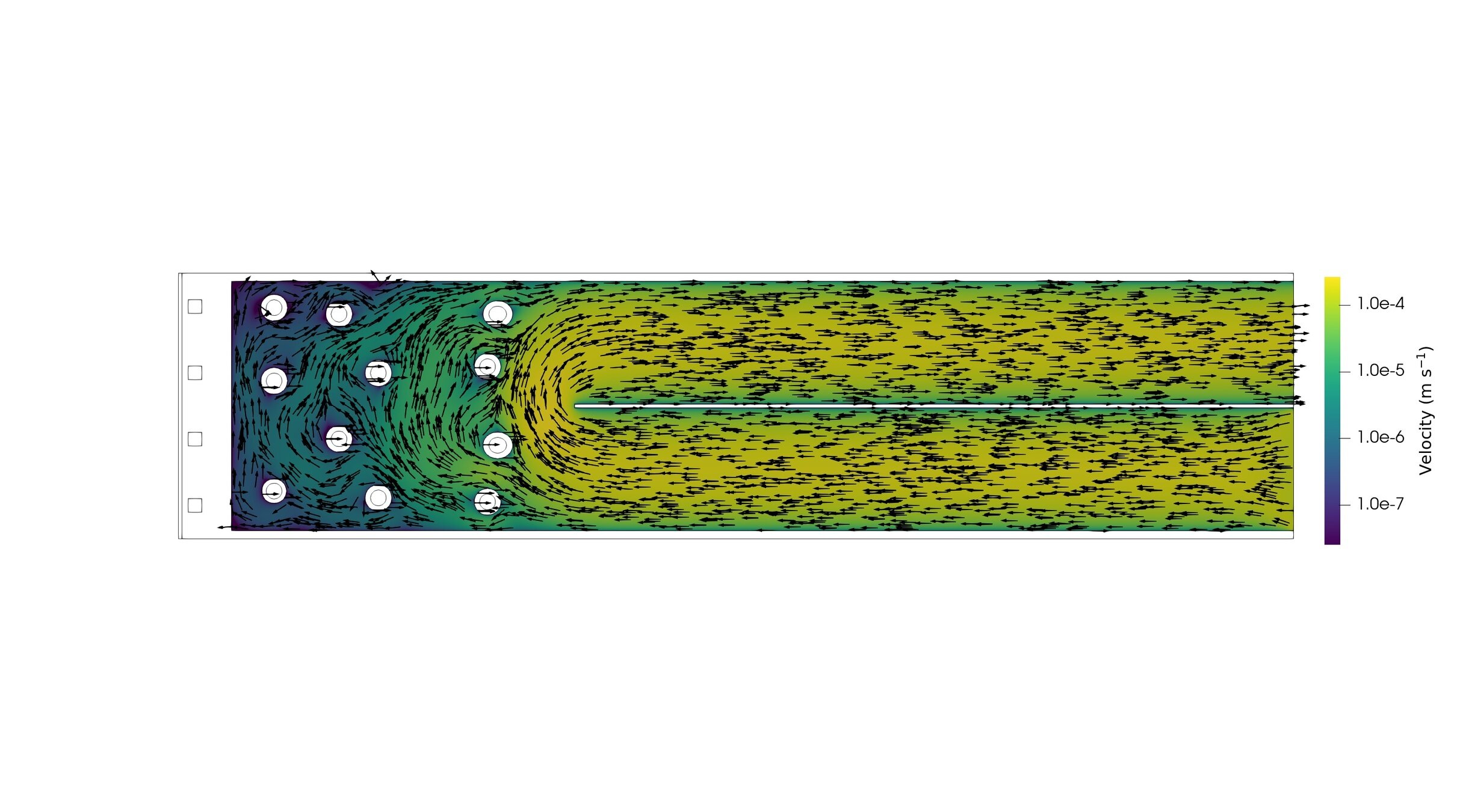
4) Fluid dynamics
5) H transport
How to handle large models
x 10,000
💡Build a surrogate model!
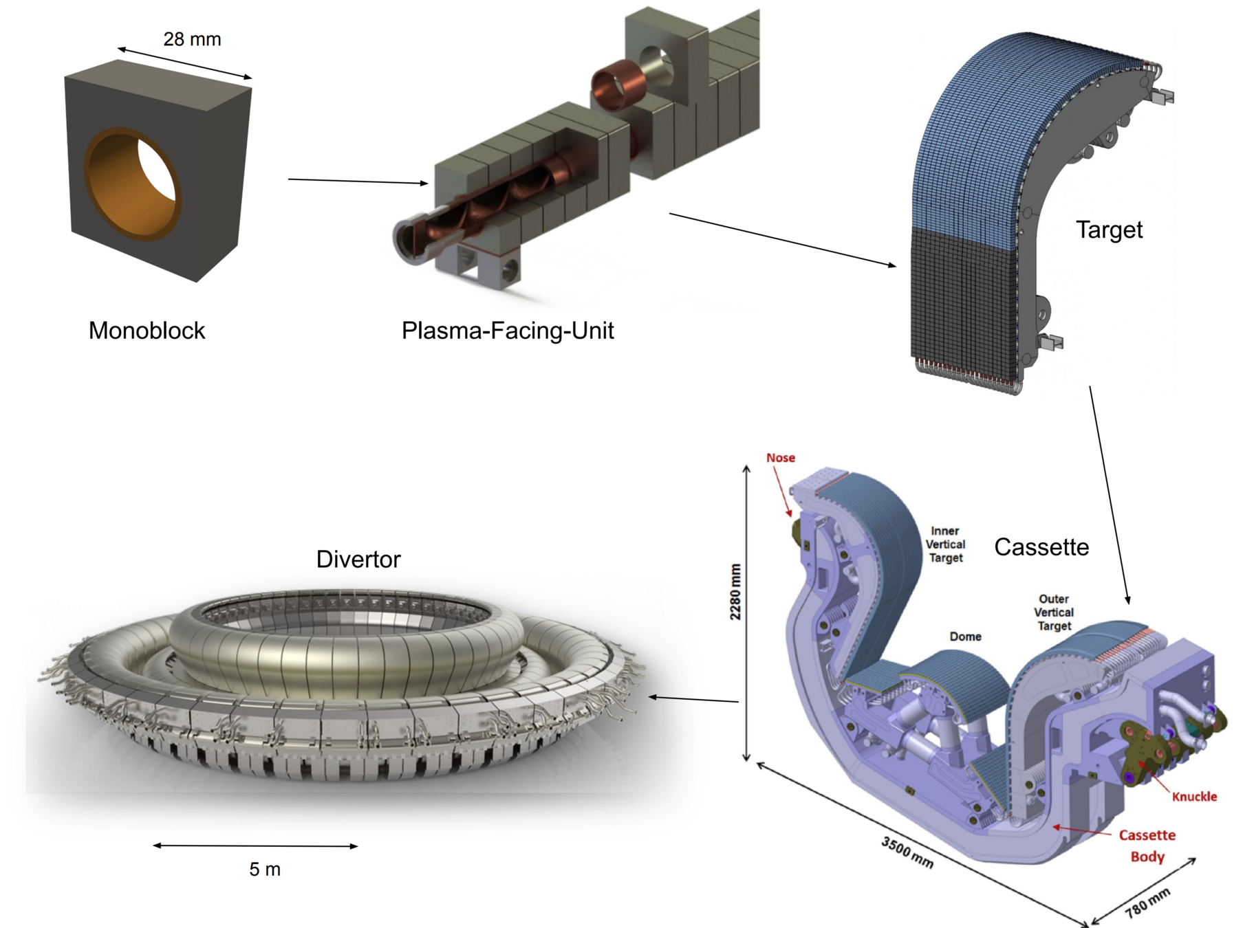
What is the inventory of the whole divertor?
Large problem
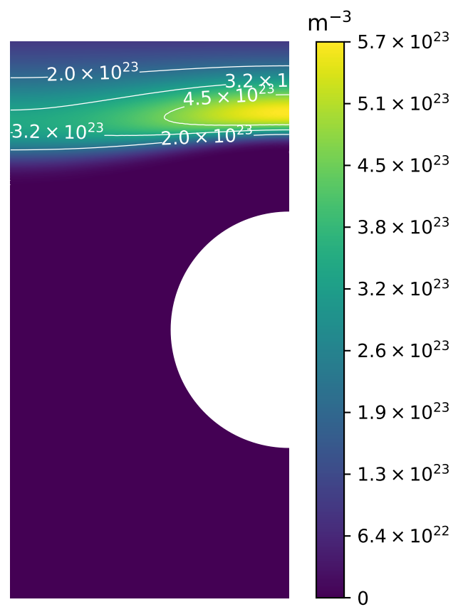
A monoblock surrogate model
At
t = 10^7 \, \mathrm{s}
\mathrm{inventory} = \int c \, dV
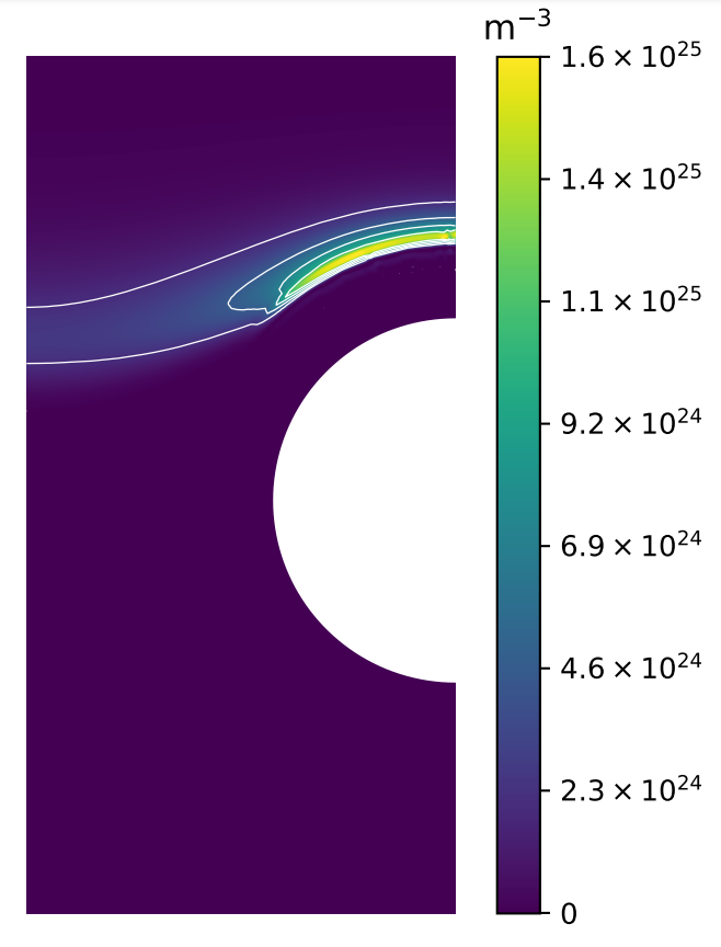
T_\mathrm{surface} = 700 \, \mathrm{K}
c_\mathrm{m} = 10^{21} \, \mathrm{H\,m^{-3}}
c_\mathrm{m} = 10^{20} \, \mathrm{H\,m^{-3}}
T_\mathrm{surface} = 1000 \, \mathrm{K}
A monoblock surrogate model
+
+
\( T_\mathrm{surface} \) (K)
\( c_\mathrm{surface} \) (\(\mathrm{m}^{-3}\))
A monoblock surrogate model
+
+
+
+
+
+
+
+
+
+
+
+
+
+
\( T_\mathrm{surface} \) (K)
\( c_\mathrm{surface} \) (\(\mathrm{m}^{-3}\))
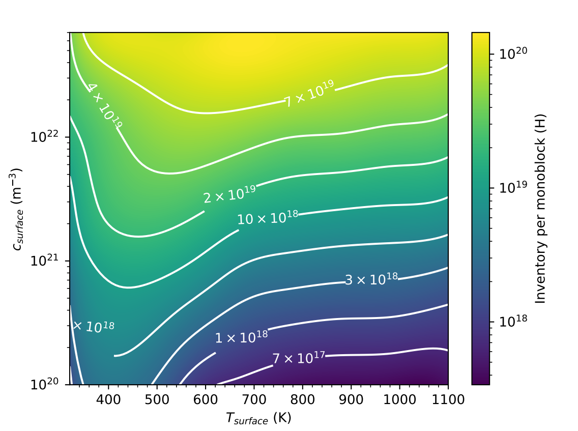
A monoblock surrogate model
\mathrm{inventory} = \int c \, dV
At
t = 10^7 \, \mathrm{s}
Gaussian Process Regression (GPR)
\( T_\mathrm{surface} \) (K)
\( c_\mathrm{surface} \) (\(\mathrm{m}^{-3}\))
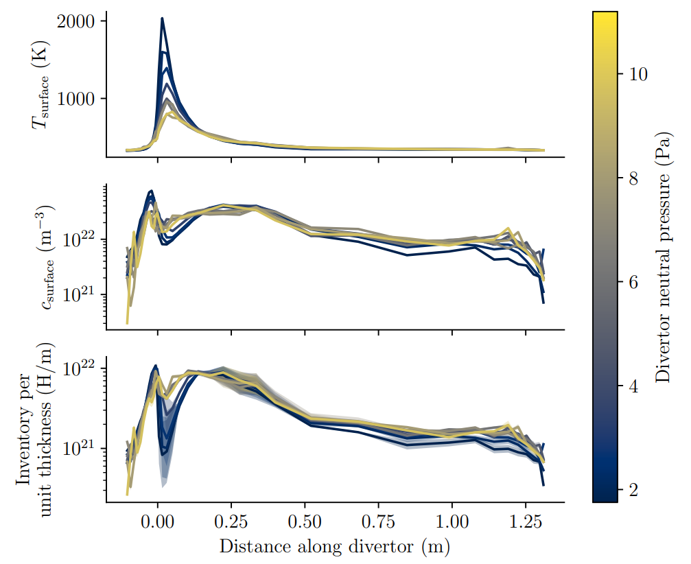
SOLPS runs: Pitts et al NME (2020)
The inventory is estimated from the surrogate model
Divertor H inventory at \( t = 10^7 \, \mathrm{s}\) is \( \approx \) 14 g
Integrate
How to handle VERY large models?
Fuel Cycle Modelling
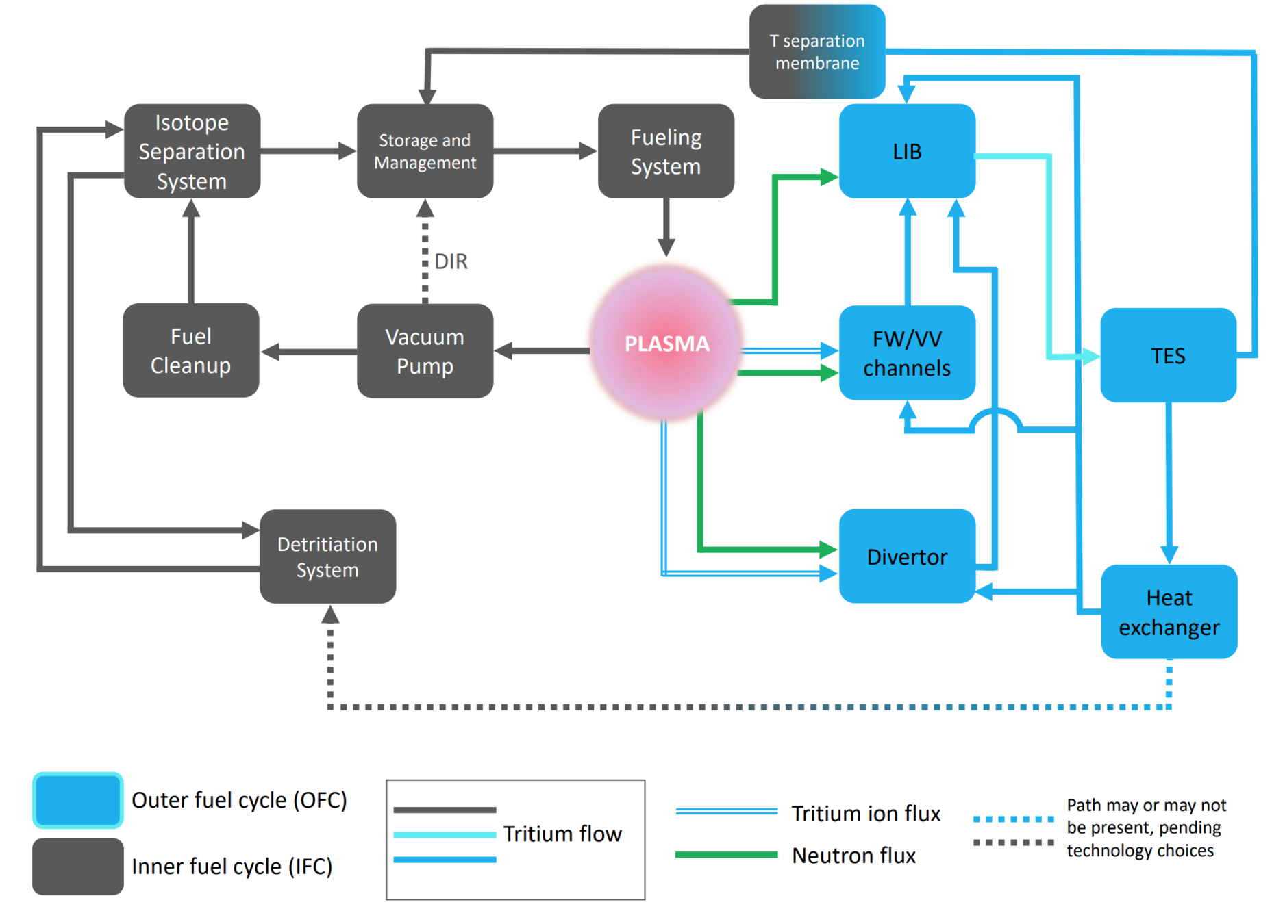
Meschini et al (submitted)
The inventory is computed in each component
BB
TES
Storage
\tau_\mathrm{BB}
\tau_\mathrm{TES}
Plasma
\frac{dI_\mathrm{BB}}{dt}=\dot{N} \cdot \mathrm{TBR} - \frac{I_\mathrm{BB}}{\tau_\mathrm{BB}} + f_{\mathrm{TES \rightarrow BB}}\frac{I_\mathrm{TES}}{\tau_\mathrm{TES}}
\frac{dI_\mathrm{TES}}{dt}= - \frac{I_\mathrm{TES}}{\tau_\mathrm{TES}} + \frac{I_\mathrm{BB}}{\tau_\mathrm{BB}}
\frac{dI_\mathrm{storage}}{dt}= - \dot{N} + f_{\mathrm{TES \rightarrow Storage}}\frac{I_\mathrm{TES}}{\tau_\mathrm{TES}}
\( I \): tritium inventory
\( \tau \): residency time
\(f\): flow fraction
The inventory is computed in each component
BB
TES
Storage
\tau_\mathrm{BB}
\tau_\mathrm{TES}
Plasma

The inventory is computed in each component
BB
TES
Storage
\tau_\mathrm{BB}
\tau_\mathrm{TES}
Plasma
Storage inventory is almost zero
The inventory is computed in each component
BB
TES
Storage
\tau_\mathrm{BB}
\tau_\mathrm{TES}
Plasma
T accumulates in storage again
The inventory is computed in each component
BB
TES
Storage
\tau_\mathrm{BB}
\tau_\mathrm{TES}
Plasma

Higher startup inventory
The inventory is computed in each component
\frac{dI_i}{dt}=\sum_{j\neq i}\left(f_{j\rightarrow i}\frac{I_j}{\tau_j}\right)-(1+\epsilon_i)\left(\frac{I_i}{\tau_i}\right)-\lambda I_i + S_i
T coming from other components
T going to other components
+ losses to environment
Radioactive decay
Production
DFT
Let's wrap everything up
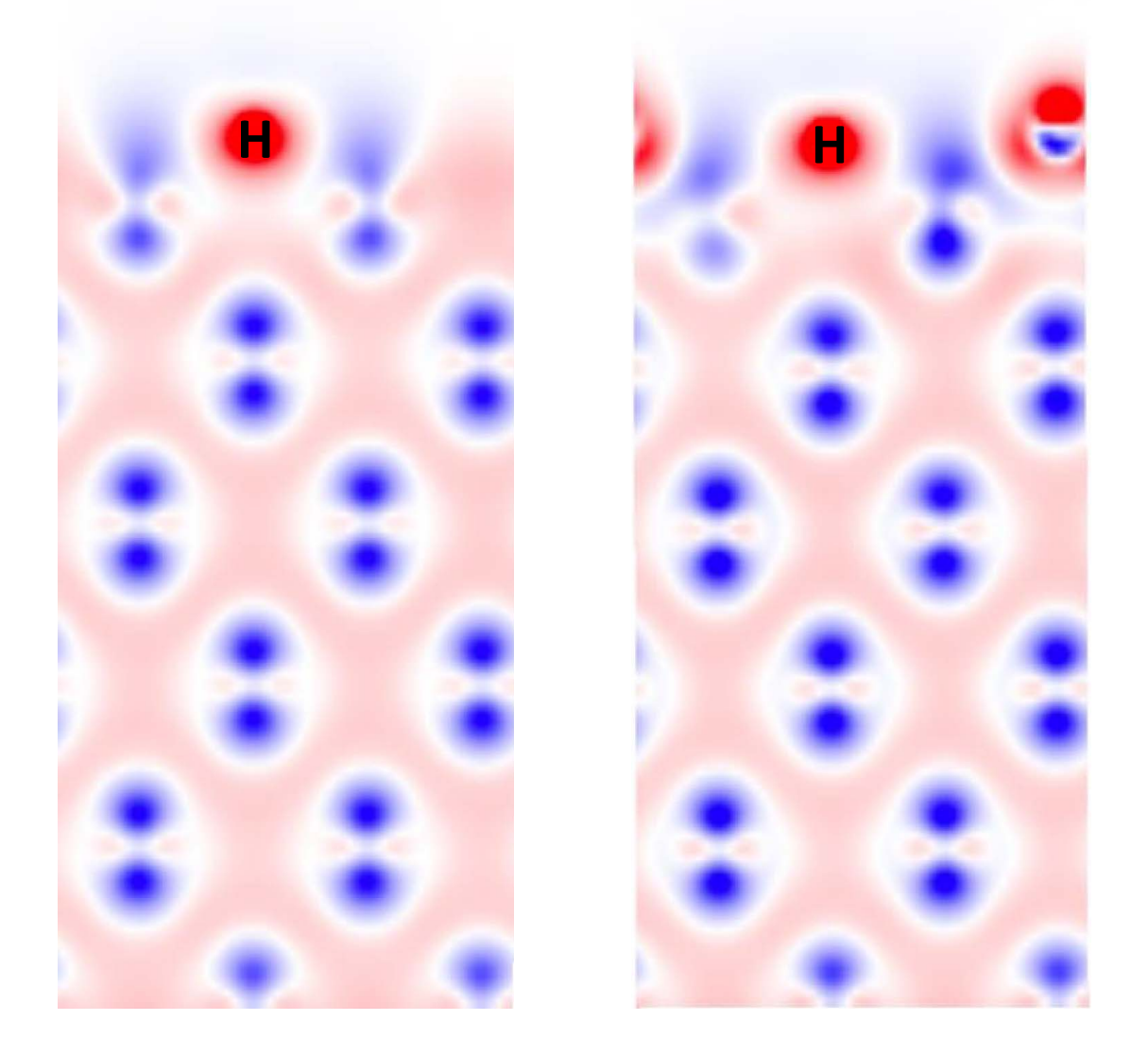
Y. Ferro et al 2023 Nucl. Fusion 63 036017
Length scale
Time scale
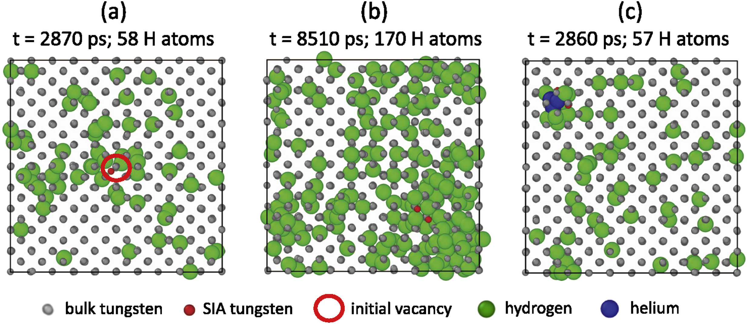
MD
Let's wrap everything up
Length scale
Time scale
DFT
potentials
Let's wrap everything up
Component scale modelling
Length scale
Time scale
MD
DFT
D, S, other coeffs.
Let's wrap everything up
Length scale
Time scale
MD
DFT
Component scale modelling
Fuel cycle modelling
Residency times, fluxes, ...
Let's wrap everything up
Length scale
Time scale
MD
DFT
Component scale modelling
Fuel cycle modelling
Abstraction
Modelling hydrogen in materials: component to reactor scale
By Remi Delaporte-Mathurin


