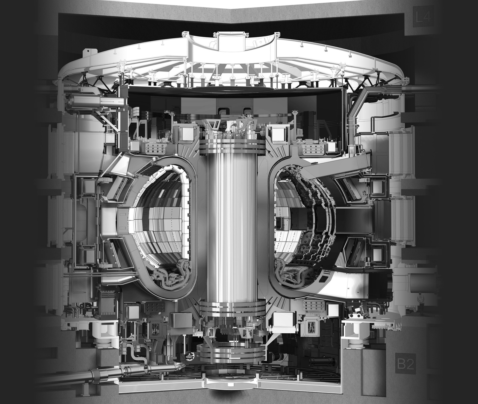
Hydrogen transport in tokamaks
Estimation of the ITER divertor tritium inventory and influence of helium exposure
Rémi Delaporte-Mathurin
17-10-2022


“I’d put my money on the Sun. What a source of power!”
Thomas Edison, 1931
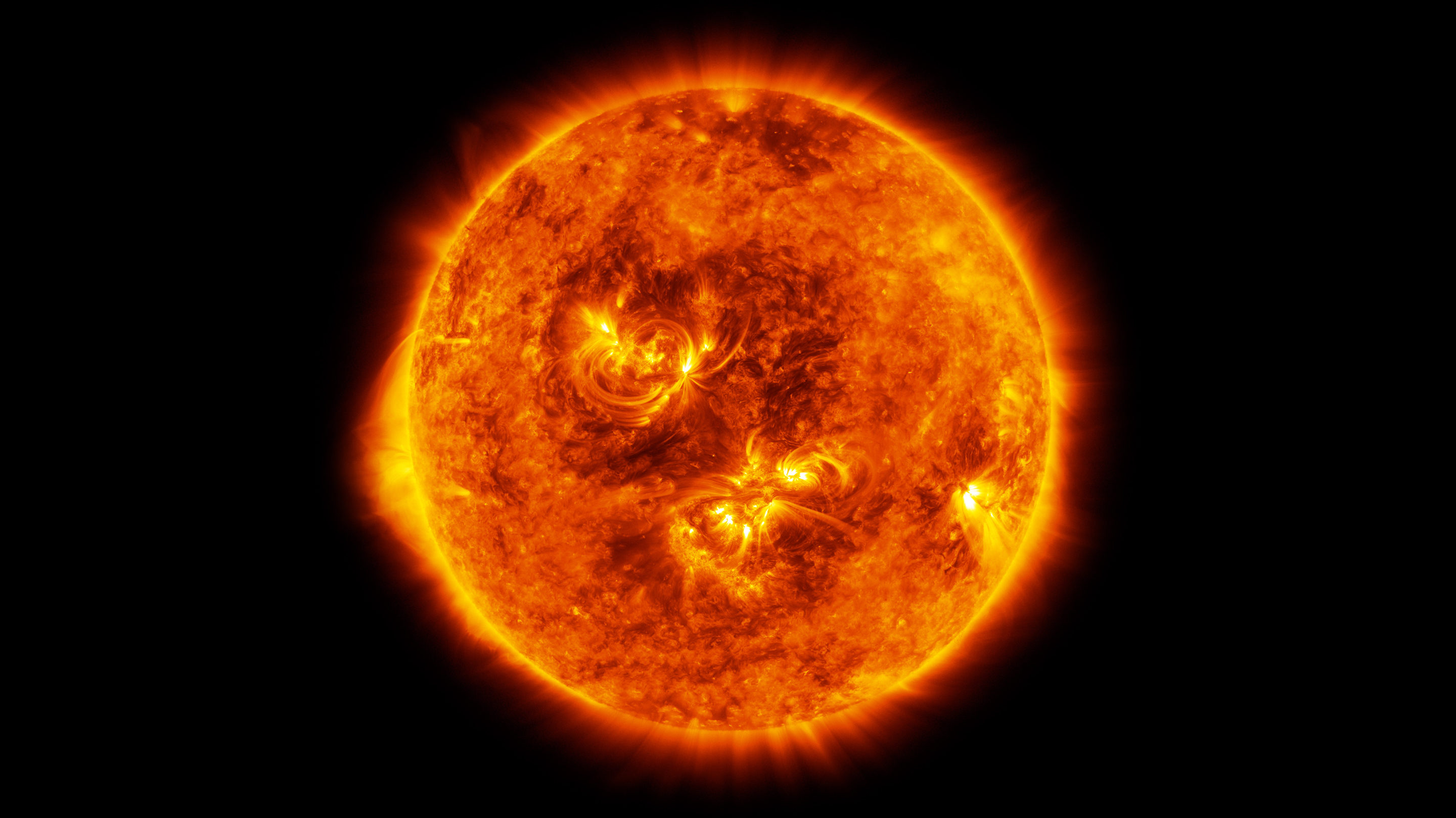
Every second:
→ Fuses 500 Mt of hydrogen
→ Produces a million times the world’s energy consumption
On Earth
Deuterium
Tritium
Neutron
Helium
✔️No CO2 emission
✔️No long lived radioactive waste
✔️Inherently safe
✔️Abundant fuel
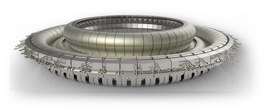
ITER
Plasma: mixture of Hydrogen (D-T) and Helium
Particle bombardment
Divertor
Why should we care?
T is rare
T is expensive
€£$
Material embrittlement
Gao et al, Nucl Fusion (2019)
What's the T inventory in the ITER divertor?
Does it remain within safety limits?
What's the influence of Helium?
T is radioactive
☢
Why should we care?
T is rare
T is expensive
£
Material embrittlement

T is radioactive
Gao et al, Nucl Fusion (2019)
What's the T inventory in the ITER divertor?
Does it remain within safety limits?
What's the influence of Helium?
Material embrittlement
Gao et al, Nucl Fusion (2019)
Fuel recycling

£
☢
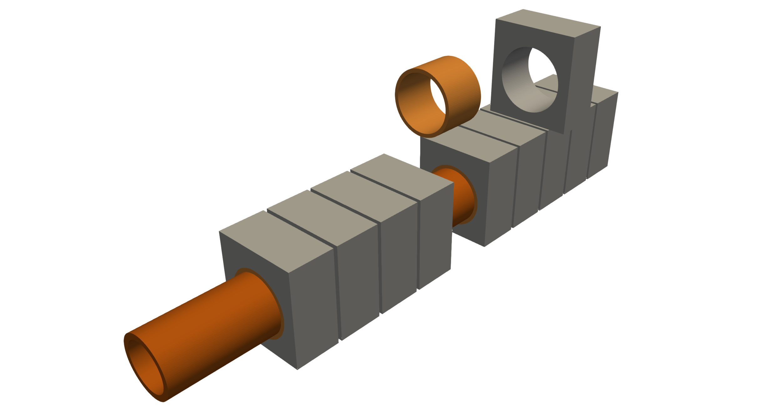
W
Cu
CuCrZr
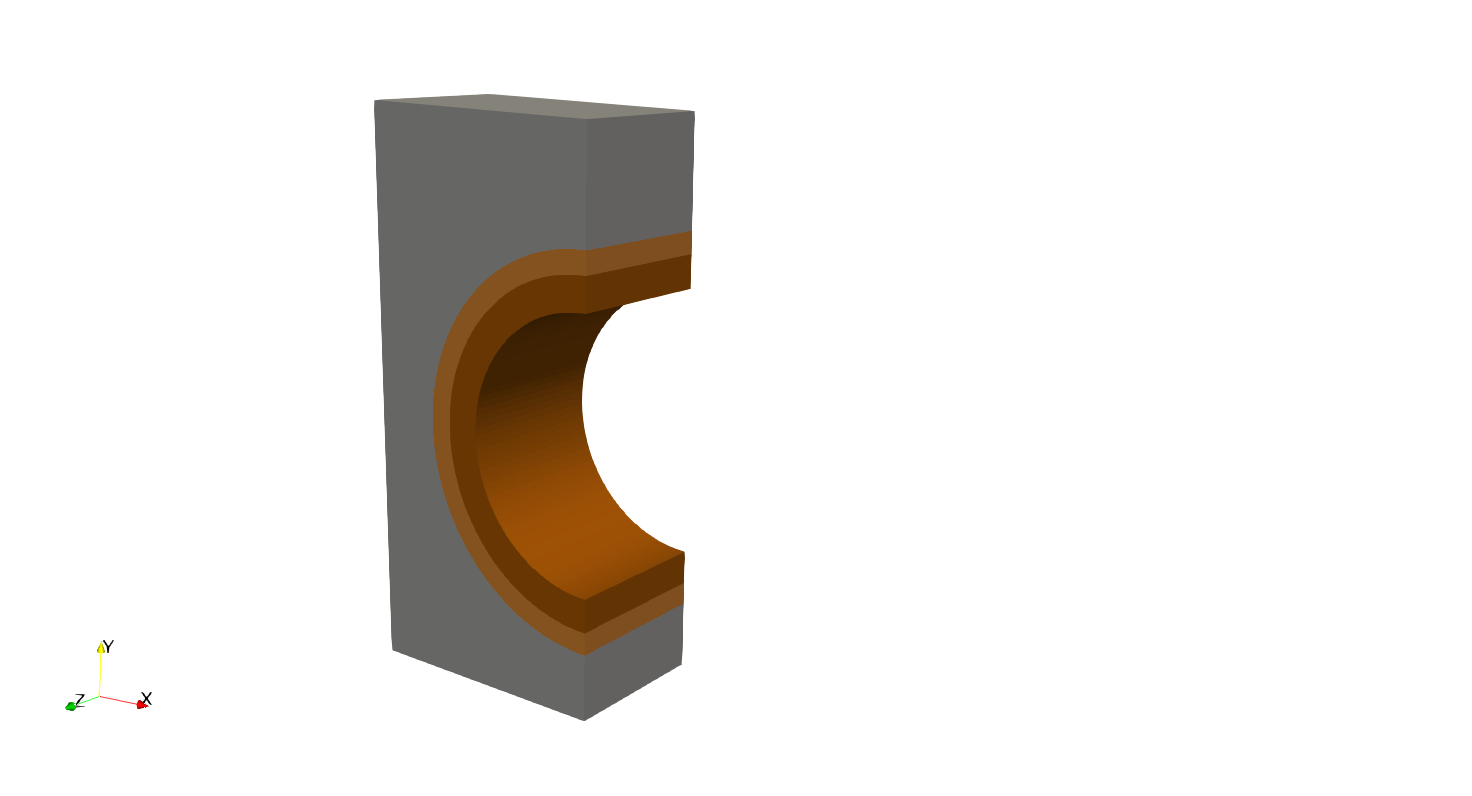
Monoblocks
W
Cu
CuCrZr
Monoblock
Top surface exposed to extreme fluxes (particle, heat)


Pressurised water convection
14 mm
Outline
- Assessment of the tritium inventory in the ITER divertor
- Models & tools
- Monoblocks
- Divertor
- Influence of helium impurities
- Helium bubble model
- Interactions with hydrogen transport
Models and tools
Hydrogen transport in metals
H transport equations
\frac{\partial c_\mathrm{m}}{\partial t} = \nabla \cdot (D \nabla c_\mathrm{m})
Fick's law
H transport equations
\textcolor{grey}{\frac{\partial \textcolor{black}{c_\mathrm{m}}}{\partial t} = \nabla \cdot (D \nabla \textcolor{black}{c_\mathrm{m}})}
c_\mathrm{m}
concentration of mobile hydrogen
Fick's law
\mathrm{(m^{-3})}
H transport equations
\textcolor{grey}{\frac{\partial c_\mathrm{m}}{\partial t} = \nabla \cdot (\textcolor{black}{D} \nabla c_\mathrm{m})}
c_\mathrm{m}
concentration of mobile hydrogen
D
diffusion coefficient
\mathrm{(m^{2} \, s^{-1})}
Fick's law
\mathrm{(m^{-3})}
H transport equations
\frac{\partial c_\mathrm{m}}{\partial t} = \nabla \cdot (D \nabla c_\mathrm{m}) - \sum_i \frac{\partial c_{\mathrm{t}, i}}{\partial t}
\frac{\partial c_{\mathrm{t}, i}}{\partial t} = k_i \ c_\mathrm{m} \ (n_i - c_{\mathrm{t}, i}) - p_i \ c_{\mathrm{t}, i}
McNabb & Foster
H transport equations
\frac{\partial c_\mathrm{m}}{\partial t} = \nabla \cdot (D \nabla c_\mathrm{m}) - \sum_i \frac{\partial c_{\mathrm{t}, i}}{\partial t}
\textcolor{grey}{\frac{\partial \textcolor{black}{c_{\mathrm{t}, i}}}{\partial t} = k_i \ c_\mathrm{m} \ (n_i - \textcolor{black}{c_{\mathrm{t}, i}}) - p_i \ \textcolor{black}{c_{\mathrm{t}, i}}}
c_{\mathrm{t}, i}
concentration of trapped hydrogen
McNabb & Foster
H transport equations
\frac{\partial c_\mathrm{m}}{\partial t} = \nabla \cdot (D \nabla c_\mathrm{m}) - \sum_i \frac{\partial c_{\mathrm{t}, i}}{\partial t}
\textcolor{grey}{\frac{\partial c_{\mathrm{t}, i}}{\partial t} = k_i \ c_\mathrm{m} \ (\textcolor{black}{n_i} - c_{\mathrm{t}, i}) - p_i \ c_{\mathrm{t}, i}}
n_i
trap concentration
c_{\mathrm{t}, i}
concentration of trapped hydrogen
McNabb & Foster
\mathrm{(m^{-3})}
H transport equations
\frac{\partial c_\mathrm{m}}{\partial t} = \nabla \cdot (D \nabla c_\mathrm{m}) - \sum_i \frac{\partial c_{\mathrm{t}, i}}{\partial t}
\textcolor{grey}{\frac{\partial c_{\mathrm{t}, i}}{\partial t} = \textcolor{black}{k_i} \ c_\mathrm{m} \ (n_i - c_{\mathrm{t}, i}) - \textcolor{black}{p_i} \ c_{\mathrm{t}, i}}
n_i
trap concentration
c_{\mathrm{t}, i}
concentration of trapped hydrogen
McNabb & Foster
k_i
trapping rate
p_i
detrapping rate
\mathrm{(m^{-3})}
\mathrm{(m^{3} \ s^{-1})}
\mathrm{(s^{-1})}
H transport equations
\frac{\partial c_\mathrm{m}}{\partial t} = \nabla \cdot (D \nabla c_\mathrm{m}) - \sum_i \frac{\partial c_{\mathrm{t}, i}}{\partial t}
\textcolor{grey}{\frac{\partial c_{\mathrm{t}, i}}{\partial t} = \textcolor{grey}{k_i} \ c_\mathrm{m} \ (n_i - c_{\mathrm{t}, i}) - \textcolor{grey}{p_i} \ c_{\mathrm{t}, i}}
Conservation of chemical potential at interfaces
\left( \frac{c_\mathrm{m}}{S}\right)^{-} = \left(\frac{c_\mathrm{m}}{S}\right)^{+}
Material 1
Material 2
\( c_\mathrm{m} \)
\( S\): solubility of H in the material
\mathrm{(m^{-3} \ Pa^{-1/2} \quad or \quad m^{-3} \ Pa^{-1})}
H transport equations
\frac{\partial c_\mathrm{m}}{\partial t} = \nabla \cdot (D \nabla c_\mathrm{m}) - \sum_i \frac{\partial c_{\mathrm{t}, i}}{\partial t}
\frac{\partial c_{\mathrm{t}, i}}{\partial t} = k_i \ c_\mathrm{m} \ (n_i - c_{\mathrm{t}, i}) - p_i \ c_{\mathrm{t}, i}
\( \textcolor{red}{T} \) : Temperature (K)
Thermally activated coefficients
\( D = D_0 \exp(-E_D / k_B \textcolor{red}{T}) \)
\( k_i = k_0 \exp(-E_k / k_B \textcolor{red}{T}) \)
\( p_i = p_0 \exp(-E_p / k_B \textcolor{red}{T}) \)
\left( \frac{c_\mathrm{m}}{S}\right)^{-} = \left(\frac{c_\mathrm{m}}{S}\right)^{+}
1800 °C
300 °C
20 MW/m2
\(k_B \): Boltzmann constant
We also need the heat equation
\rho C_p \frac{\partial T}{\partial t} = \nabla \cdot (\lambda \nabla T)
\lambda
thermal conductivity
(\mathrm{W} \, \mathrm{m}^{-1} \, \mathrm{K}^{-1})
C_p
heat capacity
(\mathrm{J} \, \mathrm{kg}^{-1} \, \mathrm{K}^{-1})
density
(\mathrm{kg}\, \mathrm{m}^{-3})
\rho
Wishlist
- Multi-materials
- Multi-dimensional
- Hydrogen transport
- Heat transfer
| 1D H transport | 2D/3D | Multi-material | Heat transfer | |
|---|---|---|---|---|
| TMAP7 | ✓ | ✓ | ||
| HIIPC | ✓ | ✓ | ||
| CRDS | ✓ | |||
| MHIMS | ✓ | |||
| TESSIM | ✓ | ✓ | ||
Wishlist
- Multi-materials
- Multi-dimensional
- Hydrogen transport
- Heat transfer
| 1D H transport | 2D/3D | Multi-material | Heat transfer | |
|---|---|---|---|---|
| TMAP7 | ✓ | ✓ | ||
| HIIPC | ✓ | ✓ | ||
| CRDS | ✓ | |||
| MHIMS | ✓ | |||
| TESSIM | ✓ | ✓ | ||
| FESTIM | ✓ | ✓ | ✓ | ✓ |
FESTIM implements these models
\rho C_p \frac{\partial T}{\partial t} = \nabla \cdot (\lambda \nabla T)
\frac{\partial c_\mathrm{m}}{\partial t} = \nabla \cdot (D \nabla c_\mathrm{m}) - \frac{\partial c_{\mathrm{t}, i}}{\partial t}
\frac{\partial c_{\mathrm{t}, i}}{\partial t} = k \ c_\mathrm{m} \ (n - c_{\mathrm{t}, i}) - p \ c_{\mathrm{t}, i}
FESTIM

Finite element
H transport
Heat transfer
Complex geometries

The finite element method
\textcolor{#fc6f00}{u_h}(x) = \sum^N_{i=1}\textcolor{#444444}{U_i} \textcolor{#2676b2}{\phi_i}(x)
\int_{\Omega} D \nabla c_\mathrm{m} \cdot \nabla v_\mathrm{m} \ dx = \int_{\Omega} \left( k c_\mathrm{m} (n - c_\mathrm{t}) - p c_\mathrm{t} \right) \ v_\mathrm{t} \ dx \quad \forall \ (v_\mathrm{m}, v_\mathrm{t}) \in \hat{V}
Steady state weak formulation:
\int_{\Omega} \frac{c_\mathrm{m} - c_{\mathrm{m}, n}}{\Delta t} \ dx + \int_{\Omega} \frac{c_\mathrm{t} - c_{\mathrm{t}, n}}{\Delta t} \ dx+ \int_{\Omega} D \nabla c_\mathrm{m} \cdot \nabla v_\mathrm{m} \ dx = -\int_{\Omega} \left( k c_\mathrm{m} (n - c_\mathrm{t}) - p c_\mathrm{t} \right) \ v_\mathrm{m} \ dx + \int_{\Omega} \left( k c_\mathrm{m} (n - c_\mathrm{t}) - p c_\mathrm{t} \right) \ v_\mathrm{t} \ dx \quad \forall \ (v_\mathrm{m}, v_\mathrm{t}) \in \hat{V}
Transient weak formulation:
In FESTIM
Type of finite elements:
- P1 (CG1) for \( c_\mathrm{m} \)
- P1 or DG1 for \( c_\mathrm{t, i} \)
FESTIM: a code verified & validated
Experimental validation
Analytical verification
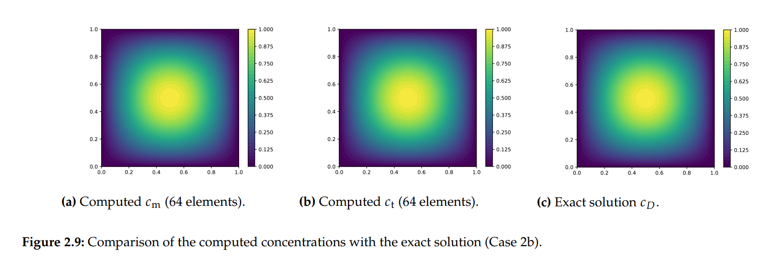
Exact
Computed concentration
Parametric optimisation technique
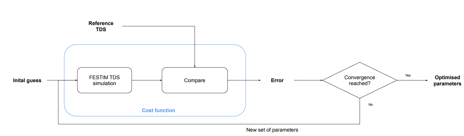
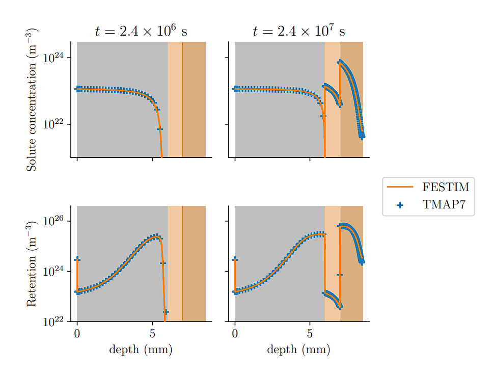
Cross-check with TMAP7
FESTIM main features
Physics
- Hydrogen diffusion
- Trapping (McNabb & Foster)
- Heat transfer
- Conservation of chemical potential
- Soret effect
Dimension
✅ 1D
✅ 2D
✅ 3D
Boundary conditions
- Imposed concentration/temperature
- Hydrogen/heat flux
- Recombination flux
- Dissociation flux
- Convective heat flux
- Sievert's law
- Plasma implantation approx.
- ...
Traps
- Time/space dependent densities
- Extrinsic traps
FESTIM: an open-source code
✅ More transparency
✅ More collaborations
✅ More flexibility
Automated documentation
FESTIM workshop

A FESTIM course to learn how to run H transport simulations
Monoblock simulations
FESTIM model
Heat flux \( \varphi_\mathrm{heat} \)
Imposed concentration
Convection
H recombination
Conservative assumptions:
- 2D
- Continuous exposure
- No desorption on gaps
Influence of mechanical fields neglected
Boundary conditions
Convective flux: \( -\lambda \nabla T \cdot n = h \ (T-T_\mathrm{coolant}) \)
Recombination flux: \( -D \nabla c_\mathrm{m} \cdot n = K_r \ c_\mathrm{m}^2 \)
Incident heat flux: \( -\lambda \nabla T \cdot n = 10 \ \mathrm{MW \ m^{-2}} \)
Heat transfer coefficient: \( h = 70,000 \ \mathrm{W \ m^{-2} \ K^{-1}} \)
Coolant temperature: \( T_\mathrm{coolant} = 323 \ \mathrm{K} \)
Recombination coefficient: \( K_r =2.9 \times 10^{-14} \ \exp{(-1.92/k_B T)}\) (\(\mathrm{m^4 \ s^{-1} }\) )
FESTIM model
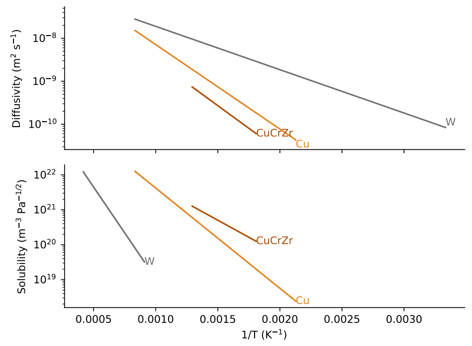
Materials properties
Trapping parameters
| W | |||||
| Cu | |||||
| CuCrZr |
3.1 \times 10^{-16}
6.0 \times 10^{-17}
1.2 \times 10^{-16}
0.42
0.39
0.20
8.4 \times 10^{12}
8.0 \times 10^{13}
8.0 \times 10^{13}
1.00
0.50
0.85
1.1 \times 10^{-3}
5.0 \times 10^{-5}
5.0 \times 10^{-5}
k_0 \, \mathrm{(m^3 \, s^{-1})}
p_0 \, \mathrm{(s^{-1})}
E_k \, \mathrm{(eV)}
E_p \, \mathrm{(eV)}
n \, \mathrm{(at \,fr)}
Simulation parameters
Thermal properties
\lambda \, \mathrm{(W \, K^{-1})}
-7.8\times 10^{-9} \, T^3 + 5\times 10^{-5} \, T^2 - 1.1\times 10^{-1} \, T + 1.8\times 10^2
-3.9\times 10^{-8} \, T^3 + 3.8\times 10^{-5} \, T^2 - 7.9\times 10^{-2} \, T + 4\times 10^2
-5.3\times 10^{-7} \, T^3 + 6.5\times 10^{-4} \, T^2 - 2.6\times 10^{-1} \, T + 3.1\times 10^2
W
14 mm
⌀ 12 mm
1.5 mm
1 mm
Geometry
Cu
CuCrZr

- Maximum 77% difference
- Equivalent trap:
- $$n=n_1 + n_2$$
- $$E_p = \frac{E_{p,1}\ n_1 + E_{p,2} \ n_2}{n} $$

Approximations
Neglecting Trap 2
A 2D model is the best trade-off between performance and accuracy


When neglecting desorption on gaps
3D = 2D
H concentration
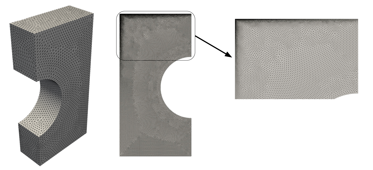
160k tetrahedrons
59k triangles
2D allows for a more refined model
ITER operations will be pulsed

Hot
Cold
The H inventory is influenced by the temperature evolution

Hot
Cold
H inventory (\(\mathrm{m^{-2}}\) )

Assuming a continuous exposure allows to have a bigger stepsize
Cycling: 1500 timesteps
Continuous: 86 timesteps
H inventory (\(\mathrm{m^{-2}}\) )
Low flux:
\( 5.0 \ \mathrm{MW \ m^{-2}} \)
\( 5.0 \times 10^{21}\ \mathrm{m^{-2} \ s^{-1}} \)
High flux:
\( 13 \ \mathrm{MW \ m^{-2}} \)
\( 1.6 \times 10^{22}\ \mathrm{m^{-2} \ s^{-1}} \)
Similar results were obtained with MHIMS
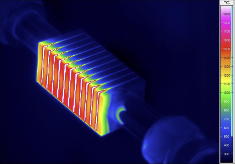
Monoblock thermal response
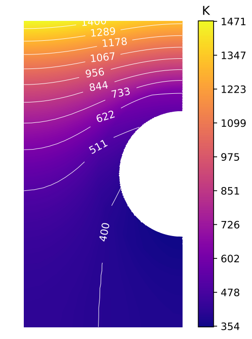
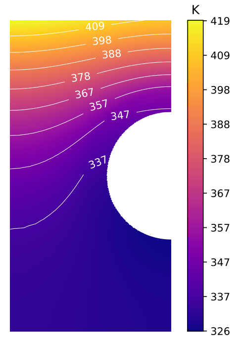
\varphi_\mathrm{heat} = 1\, \mathrm{MW \, m^{-2}}
\varphi_\mathrm{heat} = 10\, \mathrm{MW \, m^{-2}}
- High temperature gradient
- 2D temperature field
Monoblock thermal response
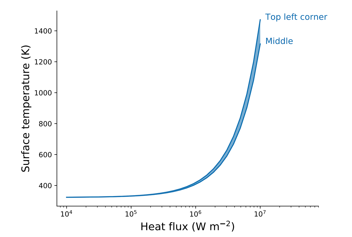
T_\mathrm{surface} = 1.1\times10^{-4} \, \varphi_\mathrm{heat} + T_\mathrm{coolant}
H concentration
At
t = 10^7 \, \mathrm{s}
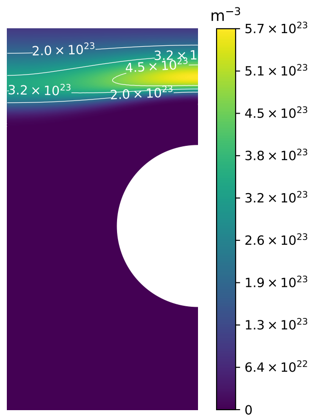
T_\mathrm{surface} = 700 \, \mathrm{K}
c_\mathrm{m} = 10^{20} \, \mathrm{H\,m^{-3}}
- Penetration front
- High retention zone in colder regions
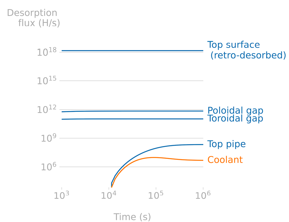
Permeation to coolant
DEMO monoblock
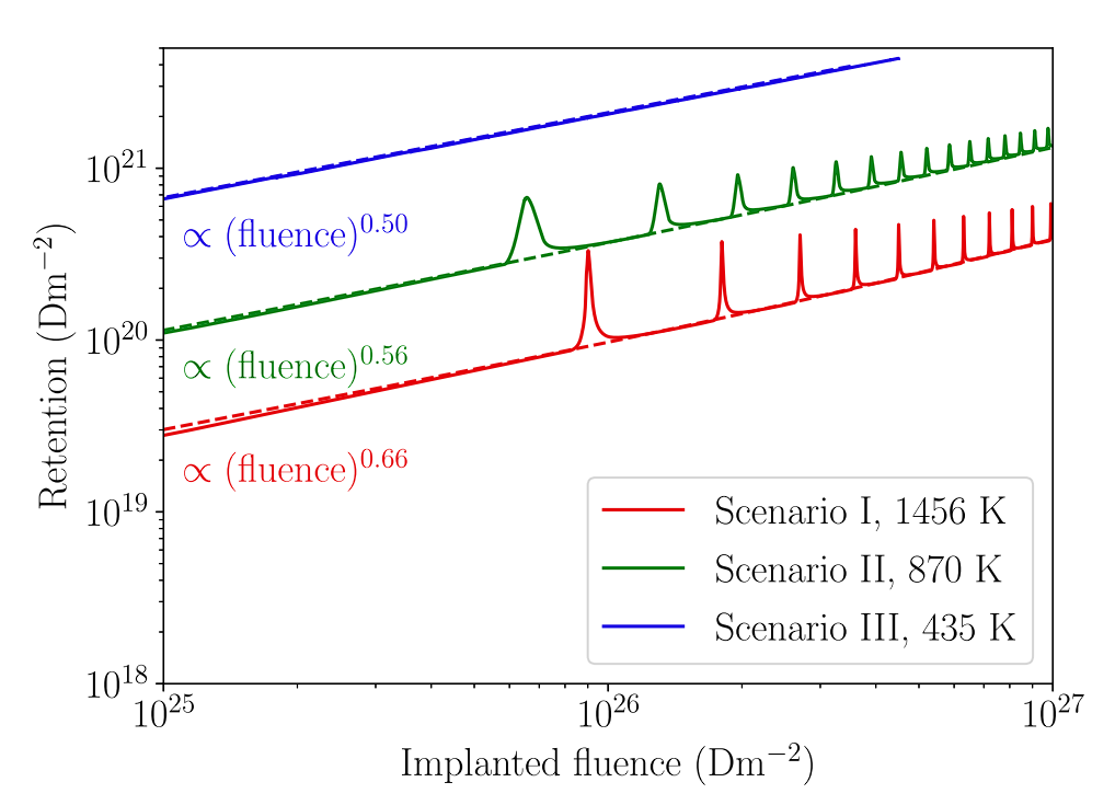
Influence of non-instantaneous recombination


wo gap and wo recombination, independent of thickness (2D)
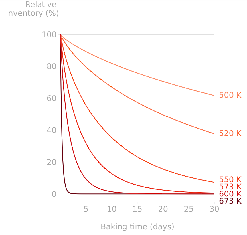
Monoblock baking
To be published
H concentration
At
t = 10^7 \, \mathrm{s}
\mathrm{inventory} = \int c \, dV
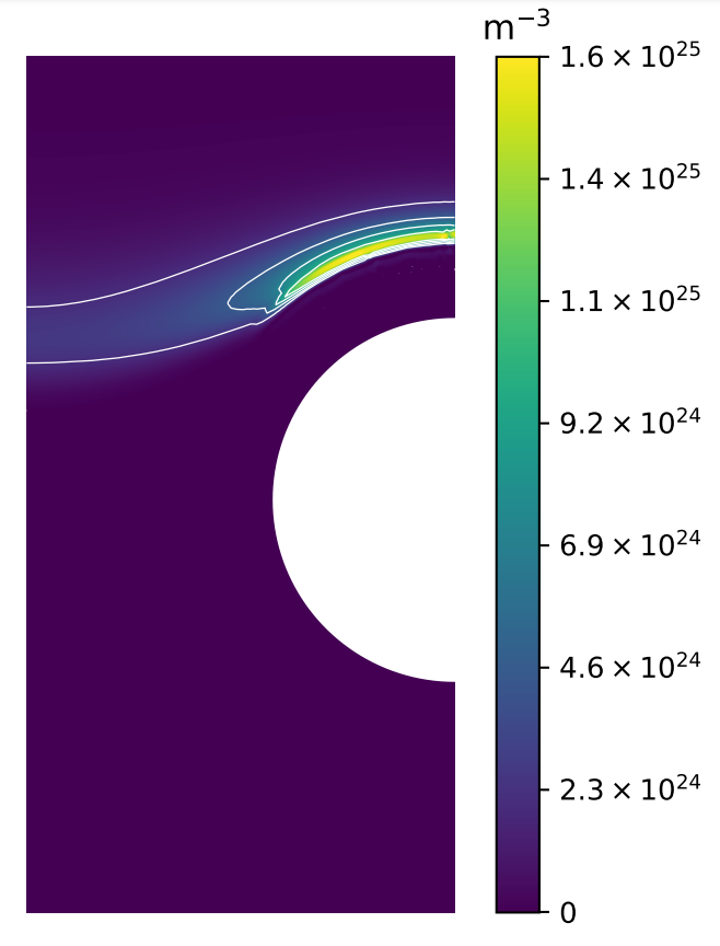
T_\mathrm{surface} = 700 \, \mathrm{K}
c_\mathrm{m} = 10^{21} \, \mathrm{H\,m^{-3}}
c_\mathrm{m} = 10^{20} \, \mathrm{H\,m^{-3}}
T_\mathrm{surface} = 1000 \, \mathrm{K}
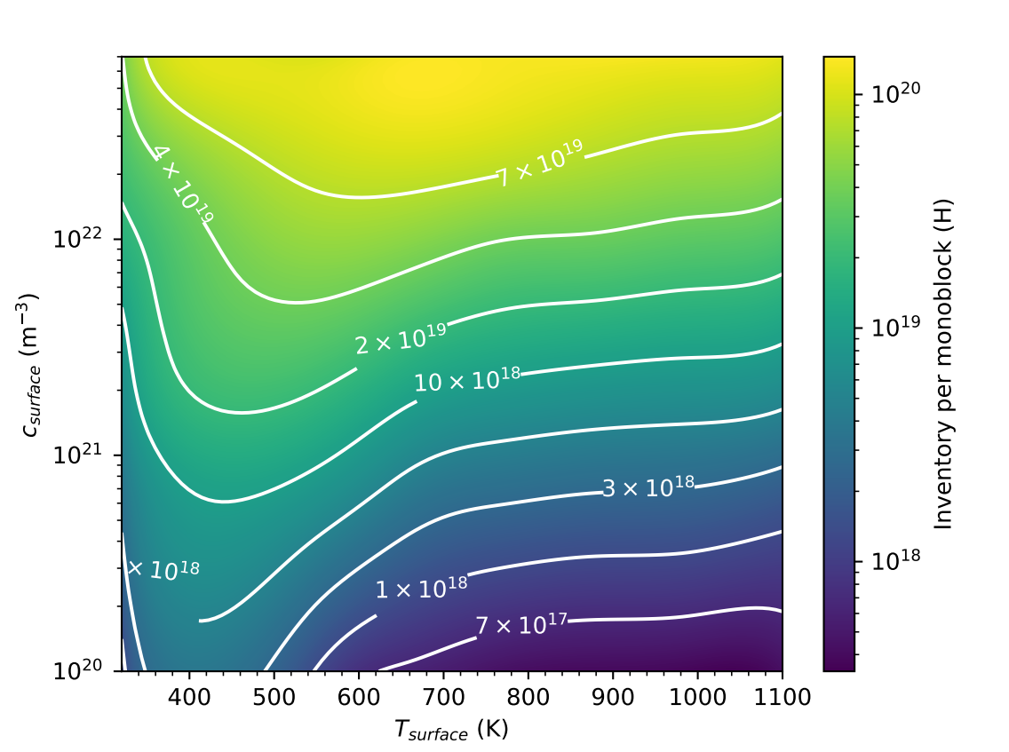
Parametric study
+
+
\( T_\mathrm{surface} \) (K)
\( c_\mathrm{surface} \) (\(\mathrm{m}^{-3}\))
Parametric study
+
+
+
+
+
+
+
+
+
+
+
+
+
+
\( T_\mathrm{surface} \) (K)
\( c_\mathrm{surface} \) (\(\mathrm{m}^{-3}\))
Parametric study
\mathrm{inventory} = \int c \, dV
At
t = 10^7 \, \mathrm{s}
Gaussian Process Regression (GPR)
\( T_\mathrm{surface} \) (K)
\( c_\mathrm{surface} \) (\(\mathrm{m}^{-3}\))
Gaussian process regression
https://juanitorduz.github.io/gaussian_process_reg/
Parametric study
Monoblock behaviour law
\mathrm{inventory} = \int c \, dV
At
t = 10^7 \, \mathrm{s}
Rapid assessment of monoblock inventories
\( c_\mathrm{surface} \) (\(\mathrm{m}^{-3}\))
\( T_\mathrm{surface} \) (K)
c_\mathrm{surface} = \frac{\varphi_\mathrm{imp} \ R_p}{D(T)}
\varphi_\mathrm{imp} \ R_p
\varphi_\mathrm{heat}
+
+
+
+
+
+
+
+
+
+
A better behaviour law
Instantaneous recombination
✔️Non homogeneous surface temperature
✔️Non homogeneous surface concentration
❌Only works for instantaneous recombination
c_\mathrm{surface} = \frac{\varphi_\mathrm{imp} \ R_p}{D(T)} + \sqrt{\frac{\varphi_\mathrm{imp}}{K_r(T)}}
R_p
\varphi_\mathrm{heat}
+
+
+
+
+
+
+
+
+
+
A better behaviour law
Non-instantaneous recombination
✔️Non homogeneous surface temperature
✔️Non homogeneous surface concentration
✔️Non-instantaneous recombination
❌3 independent variables
+
\varphi_\mathrm{imp}
A better behaviour law
Automatic sampling
Scaling up to the divertor?
Inner Vertical Target
Inner Strike Point
Outer Strike Point
Outer Vertical Target
Dome
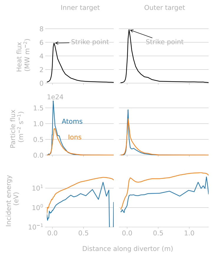
Converting plasma inputs...
T_\mathrm{surface} = 1.1\times10^{-4} \, \varphi_\mathrm{heat} + T_\mathrm{coolant}


Heat flux from SOLPS
Shot #2399
Plasma codes
\frac{\partial n}{\partial t}+\vec{\nabla} \cdot\left(n u \vec{b}+n \vec{v}_{\perp}\right)=S^n
\begin{aligned}
\frac{\partial n u}{\partial t} &+\vec{\nabla} \cdot\left(n u\left(u \vec{b}+\vec{v}_{\perp}\right)\right) \\
&=-\nabla_{\|}\left(\frac{n T_{\mathrm{i}}}{m_{\mathrm{i}}}\right)+\frac{q_{\mathrm{i}} n E_{\|}}{m_{\mathrm{i}}}+\frac{R_{\mathrm{ei}}}{m_{\mathrm{i}}}+\vec{\nabla} \cdot\left(v n \vec{\nabla}_{\perp} u\right)+S^{n u}
\end{aligned}
\begin{gathered}
\frac{\partial}{\partial t}\left(\frac{3}{2} n T_{\mathrm{i}}+\frac{1}{2} m_{\mathrm{i}} n u^2\right)+\vec{\nabla} \cdot\left(\left(\frac{5}{2} n T_{\mathrm{i}}+\frac{1}{2} m_{\mathrm{i}} n u^2\right)\left(u \vec{b}+\vec{v}_{\perp}\right)\right) \\
=\vec{\nabla} \cdot\left(\kappa_{\mathrm{i}} \nabla_{\|} T_{\mathrm{i}} \vec{b}+\chi n \vec{\nabla}_{\perp} T_{\mathrm{i}}+v n \vec{\nabla}_{\perp}\left(\frac{1}{2} m_{\mathrm{i}} u^2\right)\right) \\
\quad+q_{\mathrm{i}} n u E_{\|}+R_{\mathrm{ei}} u+Q_{\mathrm{ei}}+S^{E \mathrm{i}}
\end{gathered}
\begin{aligned}
&\frac{\partial}{\partial t}\left(\frac{3}{2} n T_{\mathrm{e}}\right)+\vec{\nabla} \cdot\left(\left(\frac{5}{2} n T_{\mathrm{e}}\right)\left(u \vec{b}+\vec{v}_{\perp}\right)\right) \\
&=\vec{\nabla} \cdot\left(\kappa_{\mathrm{e}} \nabla_{\|} T_{\mathrm{e}} \vec{b}+\chi n \vec{\nabla}_{\perp} T_{\mathrm{e}}\right)-e n u E_{\|}-R_{\mathrm{e} i} u-Q_{\mathrm{ei}}+S^{E \mathrm{e}}
\end{aligned}
Mass transport
Momentum
Ions energy \(T_\mathrm{i}\)
Electrons energy \(T_\mathrm{e}\)
\( n \): density
\( u \): velocity
Surface concentration can be estimated
Implantation depth \(R_p\)
Depth
Concentration
$$\varphi_\mathrm{imp}$$
$$\varphi_\mathrm{diff}$$
$$\varphi_\mathrm{desorption}$$
$$\varphi_\mathrm{imp} = \varphi_\mathrm{desorption} + \varphi_\mathrm{diff} $$
When \(\varphi_\mathrm{diff} \ll \varphi_\mathrm{desorption} \rightarrow c_\mathrm{max} = \frac{\varphi_\mathrm{imp} \, R_p }{D}\)
\( c_\mathrm{max}\)
Converting plasma inputs...
T_\mathrm{surface} = 1.1\times10^{-4} \, \varphi_\mathrm{heat} + T_\mathrm{coolant}
R_{p, \, i} = R_{p, \, i}(E_\mathrm{particle, \, i})
c_\mathrm{surface} = \frac{\textcolor{#fd9b21}{\varphi_\mathrm{ions} \, R_{p, \, \mathrm{ions}}} + \textcolor{#3c78d8}{\varphi_\mathrm{atoms} \, R_{p \, \mathrm{atoms}} }}{D(T_\mathrm{surface})}
Implantation range and reflection coeff. are obtained from SRIM


Use of SRIM is questionable here...
\varphi_\mathrm{imp} = (1 - r) \ \varphi_\mathrm{incident}

The flux of He is \( \approx \) 1 % of that of D
...to divertor inventory
\varphi_\mathrm{heat}
\varphi_\mathrm{particle}
T_\mathrm{surface}
Monoblock inventory
c_\mathrm{surface}
E_\mathrm{particle}
c_\mathrm{surface} = \frac{\varphi_\mathrm{ions} \, R_{p, \, \mathrm{ions}} + \varphi_\mathrm{atoms} \, R_{p \, \mathrm{atoms}}}{D(T_\mathrm{surface})}
T_\mathrm{surface} = 1.1\times10^{-4} \, \varphi_\mathrm{heat} + T_\mathrm{coolant}
+
Divertor inventory


Exposure conditions can be obtained for several divertor pressures
SOLPS runs: Pitts et al NME (2020)
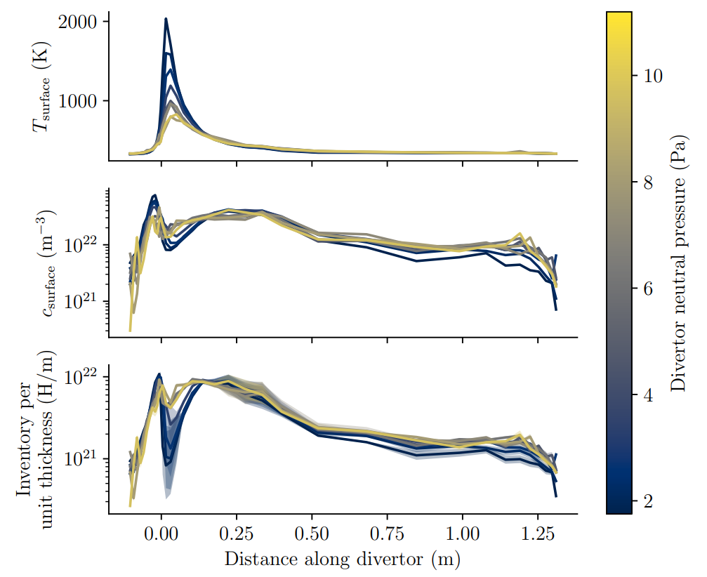
The inventory is estimated from the surrogate model
SOLPS runs: Pitts et al NME (2020)
- The strike point is not the maximum H inventory
- The total divertor inventory can be computed
$$\mathrm{inv}_\mathrm{divertor} = N_\mathrm{cassettes} ( N_\mathrm{PFU-IVT} \int \mathrm{inv}_\mathrm{IVT} (x) dx + $$
$$N_\mathrm{PFU-OVT} \int \mathrm{inv}_\mathrm{OVT} (x) dx )$$
The inventory is estimated from the surrogate model
SOLPS runs: Pitts et al NME (2020)
- The strike point is not the maximum H inventory
- The total divertor inventory can be computed
$$\mathrm{inv}_\mathrm{divertor} = 54 ( 16 \int \mathrm{inv}_\mathrm{IVT} (x) dx + $$
$$22 \int \mathrm{inv}_\mathrm{OVT} (x) dx )$$
The inventory is estimated from the surrogate model
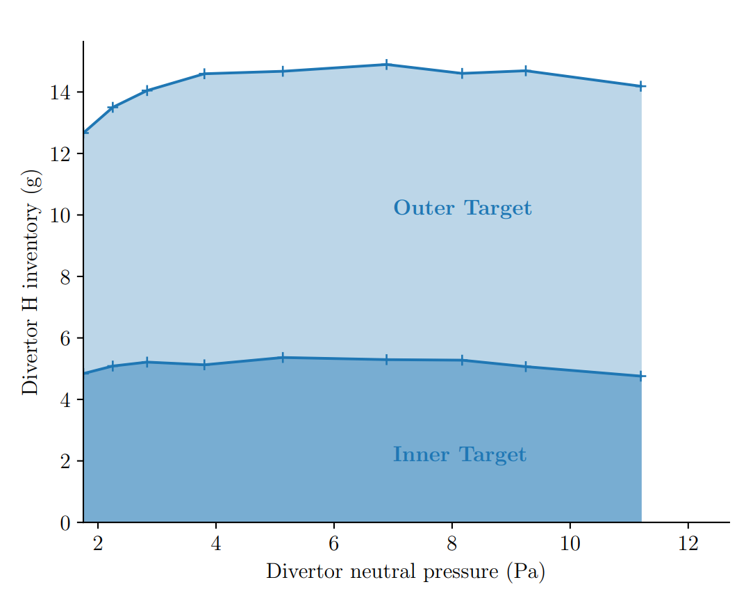
Divertor H inventory (g) at \( t = 10^7 \, \mathrm{s}\)
Safety limit \( = \) 700 g of tritium
\( \max \approx \) 2 % limit ✅
ITER divertor inventory
Safety limit \( = \) 700 g of tritium
\( \max \approx \) 2 % limit ✅
Assuming 50% T
\( \approx \) 1% limit ✅
ITER divertor inventory
Divertor H inventory (g) at \( t = 10^7 \, \mathrm{s}\)
Neglecting trap 2
Influence of helium on hydrogen transport

Why should we care?
Why should we care?
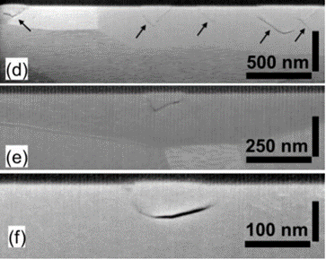
Bubbles


Tungsten fuzz
Thermo-mechanical properties
Tritium production
Hydrogen transport
Sources of helium

Neutronics monoblock simulations with OpenMC
500 MW of fusion power
\(\approx 10^{20} \mathrm{n/s} \)
500 MW of fusion power
\(\approx 10^{20} \mathrm{n/s} \)
Energy released by 1 DT reaction:
\(17.58 \ \mathrm{MeV} = 2.81 \times 10^{-12} \ \mathrm{J}\)
Tally (n,Xa) reaction

DT neutron source energy spectrum

He generation distribution
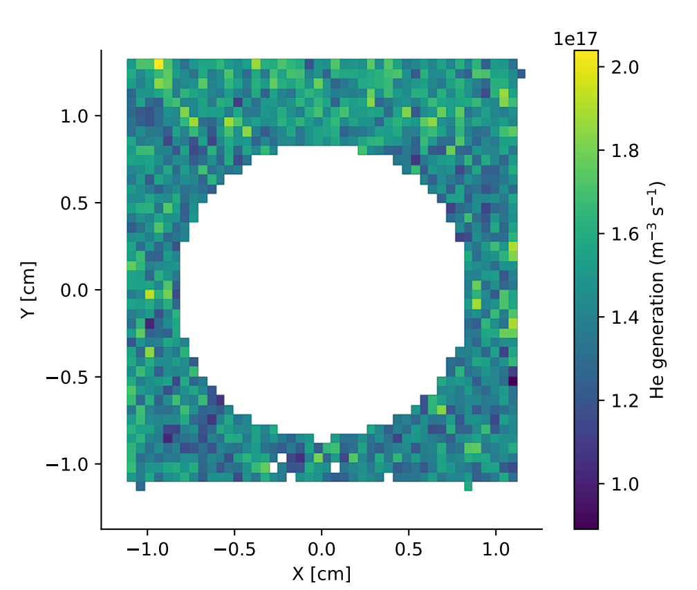
Standard deviation


Neutronic heating
Todo: assess influence of this on the thermals
Sources of helium

Tritium decay simulations with FESTIM
Neutronics monoblock simulations with OpenMC
Tritium decay
\textcolor{grey}{\frac{\partial c_\mathrm{m}}{\partial t} = \nabla \cdot (D \nabla c_\mathrm{m}) - \frac{\partial c_{\mathrm{t}, i}}{\partial t}} - \lambda c_\mathrm{m}
\textcolor{grey}{\frac{\partial c_{\mathrm{t}, i}}{\partial t} = k \ c_\mathrm{m} \ (n - c_{\mathrm{t}, i}) - p \ c_{\mathrm{t}, i}} - \lambda c_{\mathrm{t}, i}
Decay constant \( \lambda = 1.77 \times 10^{-9} \ \mathrm{s}^{-1}\)
Decay source for Helium: \( \lambda \sum c_i \)
Sources of helium

Tritium decay simulations with FESTIM
Neutronics monoblock simulations with OpenMC
→ Focus on direct implantation

He\(_1\)
He\(_2\)
He\(_4\)
He\(_3\)
V\(_1\)He\(_7\)
V\(_1\)He\(_8\)
V\(_1\)He\(_9\)
V\(_1\)He\(_{10}\)
Our clustering scheme
Trap mutation
or
self-trapping
\( \frac{\partial c_1}{\partial t} = \nabla \cdot (D_1 \nabla c_1) + P_1 - 2 k^+_{1, 1} c_1^2 - \sum\limits_{i=2}^{6}k_{1,i}^+ c_1 c_i - \langle k_b^+\rangle c_1 c_b \)
$$ \vdots $$
\( \frac{\partial c_6}{\partial t} = \nabla \cdot (D_6 \nabla c_6) - k^+_{1, 6} c_1 c_6 + k_{1,5}^+ c_1 c_{5} \)
\( \frac{\partial c_b}{\partial t} = k_{1,6}^+ c_1 c_{6} \)
\(\frac{\partial \langle i_b \rangle c_b}{\partial t} = 7 k_{1, 6}^+ c_1 c_6 + \langle k_b^+ \rangle c_1 c_b \)
Our clustering scheme
average clustering rate in bubbles
\( \langle k_b^+ \rangle = 4 \pi D_1 (r_1 + \langle r_b \rangle)\)
average bubble radius
\( \langle r_b \rangle = r_{\mathrm{He}_0\mathrm{V}_1} + \left( \frac{3}{4\pi} \frac{a_0^3}{2} \frac{\langle i_b \rangle}{4} \right)^{1/3} - \left( \frac{3}{4\pi} \frac{a_0^3}{2} \right)^{1/3}\)
Only 8 equations:
Let's consider the following reactions
\mathrm{He}_x + \mathrm{He}_1 \xrightleftharpoons[]{} \mathrm{He}_{x+1}
\mathrm{He}_x\mathrm{V}_y \rightarrow \mathrm{He}_{x}\mathrm{V}_{y+1} + \mathrm{I}_1
Helium clustering (or emission)
Trap mutation
\mathrm{A} + \mathrm{B} \xrightleftharpoons[k^-]{k^+} \mathrm{AB}
\frac{\partial c_\mathrm{AB}}{\partial t} = -\frac{\partial c_\mathrm{A}}{\partial t} = -\frac{\partial c_\mathrm{B}}{\partial t} = k^+ c_\mathrm{A} c_\mathrm{B} - k^- c_\mathrm{AB}
k^+ = (r_A + r_B) (D_A + D_B)
k^- = \rho k^+ e^{-E_b/k_B T}
For each reaction
\frac{\partial c_i}{\partial t} = \nabla \cdot (D_i \nabla c_i) + P_i + R_i(c_1, c_2, \cdots, c_N)
3-species model:
Rate constants:
N-species model:
Diffusion coefficients
Capture radii
Diffusion
Production
Reaction
Binding energy
0 = D_i \nabla^2 n_i(r) \quad \mathrm{s.t.} \quad n_i(r_{i,j}) = 0 \quad \& \quad n_i(\infty) = c_i
n_i(r) = c_i \ (1-\frac{r_{i,j}}{r})
I_{i,j} = \oint_S D_i \frac{d\ n_i(r)}{dr}\Bigr|_{\substack{r=r_{i,j}}} = 4\pi \ r_{i,j} \ D_i \ c_i
k_{i,j}^+ = \frac{I_{i,j}}{c_i} = 4 \pi \ r_{i,j} \ D_i
Derivation of the forward reaction rate
\(n_i\): local concentration
\(c_i \): mean concentration
\( r_{i,j} = r_i + r_j \): coordinate where the reaction happens (capture radii)

$$c_i$$
$$j$$
in spherical coordinates
2 diffusive species from superpostion principle:
$$k_{i,j}^+ = 4\pi \ r_{i,j} \ (D_i + D_j) $$
Issue #1: Too many equations
\( \frac{\partial c_1}{\partial t} = \nabla \cdot (D_1 \nabla c_1) + P_1 - 2 k^+_{1, 1} c_1^2 - \sum\limits_{i=2}^\infty k_{1,i}^+ c_1 c_i \)
$$ \vdots $$
\( \frac{\partial c_i}{\partial t} = \nabla \cdot (D_i \nabla c_i) - k^+_{1, i} c_1 c_i + k_{1,i-1}^+ c_1 c_{i-1} \)
$$ \vdots $$
\( \frac{\partial c_{N}}{\partial t} =\) \(- k^+_{1, N} c_1 c_{N}\) \( + k_{1,N-1}^+ c_1 c_{N-1} \)
\( \frac{\partial c_{N+1}}{\partial t} =\) \(- k^+_{1, N+1} c_1 c_{N+1}\) \( + k_{1,N}^+ c_1 c_{N} \)
\( \frac{\partial c_{N+2}}{\partial t} =\) \(- k^+_{1, N+2} c_1 c_{N+2}\) \( + k_{1,N+1}^+ c_1 c_{N+1} \)
$$ \vdots $$
💪
\( \frac{\partial c_1}{\partial t} = \nabla \cdot (D_1 \nabla c_1) + P_1 - 2 k^+_{1, 1} c_1^2 - \sum\limits_{i=2}^\infty k_{1,i}^+ c_1 c_i \)
$$ \vdots $$
\( \frac{\partial c_i}{\partial t} = \nabla \cdot (D_i \nabla c_i) - k^+_{1, i} c_1 c_i + k_{1,i-1}^+ c_1 c_{i-1} \)
$$ \vdots $$
\( \frac{\partial c_{N+1}}{\partial t} =\) \(- k^+_{1, N+1} c_1 c_{N+1}\) \( + k_{1,N}^+ c_1 c_{N} \)
\( \frac{\partial c_{N+2}}{\partial t} =\) \(- k^+_{1, N+2} c_1 c_{N+2}\) \( + k_{1,N+1}^+ c_1 c_{N+1} \)
\( \frac{\partial c_{N+3}}{\partial t} =\) \(- k^+_{1, N+3} c_1 c_{N+3}\) \( + k_{1,N+2}^+ c_1 c_{N+2} \)
$$ \vdots $$
💪
Issue #1: Too many equations
\( \frac{\partial c_1}{\partial t} = \nabla \cdot (D_1 \nabla c_1) + P_1 - 2 k^+_{1, 1} c_1^2 - \sum\limits_{i=2}^\infty k_{1,i}^+ c_1 c_i \)
$$ \vdots $$
\( \frac{\partial c_i}{\partial t} = \nabla \cdot (D_i \nabla c_i) - k^+_{1, i} c_1 c_i + k_{1,i-1}^+ c_1 c_{i-1} \)
$$ \vdots $$
\( \sum\limits_{i=N+1}^{\infty} \frac{\partial c_i}{\partial t} = k_{1,N}^+ c_1 c_{N} \)
💪
Issue #1: Too many equations
\( \frac{\partial c_1}{\partial t} = \nabla \cdot (D_1 \nabla c_1) + P_1 - 2 k^+_{1, 1} c_1^2 - \sum\limits_{i=2}^\infty k_{1,i}^+ c_1 c_i \)
$$ \vdots $$
\( \frac{\partial c_i}{\partial t} = \nabla \cdot (D_i \nabla c_i) - k^+_{1, i} c_1 c_i + k_{1,i-1}^+ c_1 c_{i-1} \)
$$ \vdots $$
\( \frac{\partial c_b}{\partial t} = k_{1,N}^+ c_1 c_{N} \)
\( c_b = \sum\limits_{i=N+1}^{\infty} c_i \) : bubble concentration
💪
Issue #1: Too many equations
\( \frac{\partial c_1}{\partial t} = \nabla \cdot (D_1 \nabla c_1) + P_1 - 2 k^+_{1, 1} c_1^2 - \sum\limits_{i=2}^{N}k_{1,i}^+ c_1 c_i - \sum\limits_{i=N+1}^\infty k_{i, 1}^+c_i c_1 \)
$$ \vdots $$
\( \frac{\partial c_i}{\partial t} = \nabla \cdot (D_i \nabla c_i) - k^+_{1, i} c_1 c_i + k_{1,i-1}^+ c_1 c_{i-1} \)
$$ \vdots $$
\( \frac{\partial c_b}{\partial t} = k_{1,N}^+ c_1 c_{N} \)
\( c_b = \sum\limits_{i=N+1}^{\infty} c_i \) : bubble concentration
💪
Issue #1: Too many equations
\( \frac{\partial c_1}{\partial t} = \nabla \cdot (D_1 \nabla c_1) + P_1 - 2 k^+_{1, 1} c_1^2 - \sum\limits_{i=2}^{N}k_{1,i}^+ c_1 c_i - \langle k_b^+\rangle c_1 c_b \)
$$ \vdots $$
\( \frac{\partial c_i}{\partial t} = \nabla \cdot (D_i \nabla c_i) - k^+_{1, i} c_1 c_i + k_{1,i-1}^+ c_1 c_{i-1} \)
$$ \vdots $$
\( \frac{\partial c_b}{\partial t} = k_{1,N}^+ c_1 c_{N} \)
\( c_b = \sum\limits_{i=N+1}^{\infty} c_i \) : bubble concentration
\( \langle k_b^+ \rangle = \left( \sum\limits_{i=N+1}^{\infty} k_ {i, 1}^+ c_i \right) / c_b\) : average clustering rate in bubbles
💪
Issue #1: Too many equations
\( c_b = \sum\limits_{i=N+1}^{\infty} c_i \) : bubble concentration
\( \langle k_b^+ \rangle = \left( \sum\limits_{i=N+1}^{\infty} k_ {i, 1}^+ c_i \right) / c_b\)
\( = \left(\sum\limits_{i=N+1}^{\infty} 4 \pi D_1 (r_1 + r_i) c_i\right) / c_b \)
💪
average clustering rate in bubbles
Issue #2: what's the value of \( \langle k_b^+ \rangle \)?
Issue #2: what's the value of \( \langle k_b^+ \rangle \)?
\( c_b = \sum\limits_{i=N+1}^{\infty} c_i \) : bubble concentration
\( \langle r_b \rangle = \left( \sum\limits_{i=N+1}^{\infty} r_ i c_i \right) / c_b\) : average bubble radius
\( \langle k_b^+ \rangle \)\( = \left( \sum\limits_{i=N+1}^{\infty} k_ {i, 1}^+ c_i \right) / c_b\)
\( = \left(\sum\limits_{i=N+1}^{\infty} 4 \pi D_1 (r_1 + r_i) c_i\right) / c_b \)
\( =4 \pi D_1 (r_1 + \langle r_b \rangle)\)
💪
average clustering rate in bubbles
\( r_i = r_{\mathrm{He}_0\mathrm{V}_1} + \left( \frac{3}{4\pi} \frac{a_0^3}{2} n_{\mathrm{V},i} \right)^{1/3} - \left( \frac{3}{4\pi} \frac{a_0^3}{2} \right)^{1/3}\)
💪
\( c_b = \sum\limits_{i=N+1}^{\infty} c_i \) : bubble concentration
\( \langle k_b^+ \rangle = 4 \pi D_1 (r_1 + \langle r_b \rangle)\) : average clustering rate in bubbles
\( \langle r_b \rangle = \left( \sum\limits_{i=N+1}^{\infty} r_ i c_i \right) / c_b\) : average bubble radius
Issue #3: what's the value of \( \langle r_b \rangle \)?
\( r_i = r_{\mathrm{He}_0\mathrm{V}_1} + \left( \frac{3}{4\pi} \frac{a_0^3}{2} \frac{i}{4} \right)^{1/3} - \left( \frac{3}{4\pi} \frac{a_0^3}{2} \right)^{1/3}\)
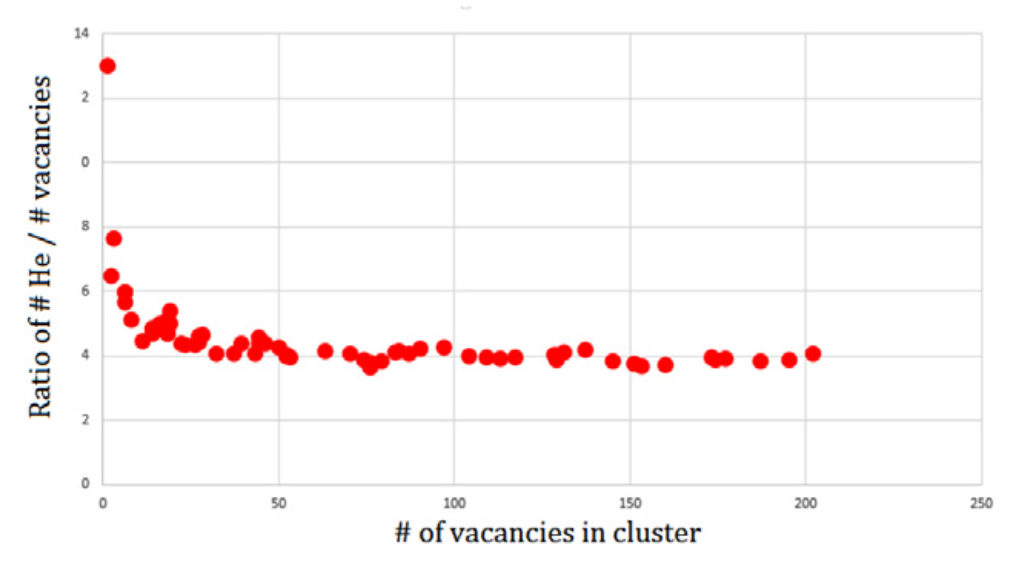
\( n_{\mathrm{V},i} = i/4 \) : 4 He per vacancy
💪
\( c_b = \sum\limits_{i=N+1}^{\infty} c_i \) : bubble concentration
\( \langle k_b^+ \rangle = 4 \pi D_1 (r_1 + \langle r_b \rangle)\) : average clustering rate in bubbles
\( \langle r_b \rangle = \left( \sum\limits_{i=N+1}^{\infty} r_ i c_i \right) / c_b\) : average bubble radius
Issue #3: what's the value of \( \langle r_b \rangle \)?
\( c_b = \sum\limits_{i=N+1}^{\infty} c_i \) : bubble concentration
\( \langle k_b^+ \rangle = 4 \pi D_1 (r_1 + \langle r_b \rangle)\) : average clustering rate in bubbles
\( \langle r_b \rangle = \left( \sum\limits_{i=N+1}^{\infty} r_ i c_i \right) / c_b\) : average bubble radius
\( \langle i_b \rangle = \left( \sum\limits_{i=N+1}^{\infty} i c_i \right) / c_b\) : average He content in bubbles
\( n_{\mathrm{V},i} = i/4 \) : 4 He per vacancy
💪
\( \langle r_b \rangle = r_{\mathrm{He}_0\mathrm{V}_1} + \left( \frac{3}{4\pi} \frac{a_0^3}{2} \frac{\langle i_b \rangle}{4} \right)^{1/3} - \left( \frac{3}{4\pi} \frac{a_0^3}{2} \right)^{1/3}\)
\( r_i = r_{\mathrm{He}_0\mathrm{V}_1} + \left( \frac{3}{4\pi} \frac{a_0^3}{2} \frac{i}{4} \right)^{1/3} - \left( \frac{3}{4\pi} \frac{a_0^3}{2} \right)^{1/3}\)
Issue #3: what's the value of \( \langle r_b \rangle \)?

\( \langle r_b \rangle = r_{\mathrm{He}_0\mathrm{V}_1} + \left( \frac{3}{4\pi} \frac{a_0^3}{2} \frac{\langle i_b \rangle}{4} \right)^{1/3} - \left( \frac{3}{4\pi} \frac{a_0^3}{2} \right)^{1/3}\)
\( \frac{\sum\limits_{i=N+1}^{\infty} i^{1/3} c_i } { c_b} \approx \left( \sum\limits_{i=N+1}^{\infty} i c_i / c_b \right)^{1/3} = \langle i_b \rangle ^{1/3}\)
When \( c_i \) has a narrow gaussian distribution (ie. \(\sigma / \mu \ll 1\) )
Sum approximation
\( \langle i_b \rangle = \left( \sum\limits_{i=N+1}^{\infty} i c_i \right) / c_b\)
\( \langle i_b \rangle c_b= \sum\limits_{i=N+1}^{\infty} i c_i \)
\(\frac{\partial \langle i_b \rangle c_b}{\partial t} = \sum\limits_{i=N+1}^{\infty} i \frac{\partial c_i}{\partial t}\)
💪
\(\frac{\partial \langle i_b \rangle c_b}{\partial t} = (N+1) k_{1, N}^+ c_1 c_N + \langle k_b^+ \rangle c_1 c_b \)
↓ trust me
\( c_b = \sum\limits_{i=N+1}^{\infty} c_i \) : bubble concentration
\( \langle k_b^+ \rangle = 4 \pi D_1 (r_1 + \langle r_b \rangle)\) : average clustering rate in bubbles
\( \langle i_b \rangle = \left( \sum\limits_{i=N+1}^{\infty} i c_i \right) / c_b\) : average He content in bubbles
Issue #4: what's the value of \( \langle i_b \rangle \)?
\( \frac{\partial c_1}{\partial t} = \nabla \cdot (D_1 \nabla c_1) + P_1 - 2 k^+_{1, 1} c_1^2 - \sum\limits_{i=2}^{N-1}k_{1,i}^+ c_1 c_i - \langle k_b^+\rangle c_1 c_b \)
$$ \vdots $$
\( \frac{\partial c_i}{\partial t} = \nabla \cdot (D_i \nabla c_i) - k^+_{1, i} c_1 c_i + k_{1,i-1}^+ c_1 c_{i-1} \)
$$ \vdots $$
\( \frac{\partial c_b}{\partial t} = k_{1,N}^+ c_1 c_{N} \)
💪
\(\frac{\partial \langle i_b \rangle c_b}{\partial t} = (N+1) k_{1, N}^+ c_1 c_N + \langle k_b^+ \rangle c_1 c_b \)
\( c_b = \sum\limits_{i=N+1}^{\infty} c_i \) : bubble concentration
\( \langle k_b^+ \rangle = 4 \pi D_1 (r_1 + \langle r_b \rangle)\) : average clustering rate in bubbles
\( \langle i_b \rangle = \left( \sum\limits_{i=N+1}^{\infty} i c_i \right) / c_b\) : average He content in bubbles
Issue #4: what's the value of \( \langle i_b \rangle \)?
Assumption time!
- Only pure He clusters are mobile
- Trap-mutation from 7 He
- Grouping starts at \( i > 6 \)
- He/V ratio: 4
- No He emission from bubbles
- Pre-existing vacancies are neglected
- We don't solve for W self-interstitials
-
Diffusion coefficients from Faney et al. Nucl. Fusion (2015)
-
Dissociation energies from Becquart et al. J. Nucl. Mater. (2010)
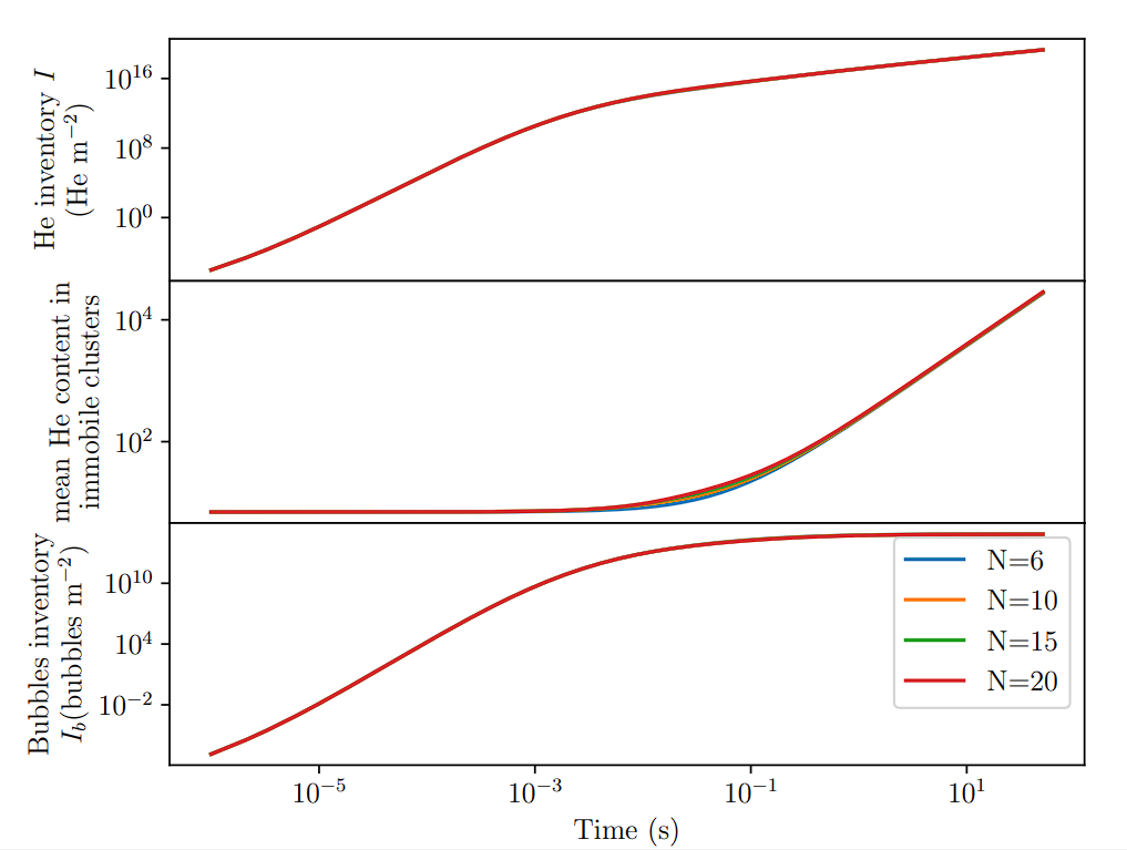
Varying the grouping threshold
Results on a half-slab case

- Helium first diffuses rapidly into the bulk
- Mobile helium is consumed to form bubbles
\(c_i = 0 \)
W
He implantation
Mobile helium
Bubbles
Retention
$$\mathrm{m}^{-3}$$
Half-slab case
- "Semi-infinite" (0.6 mm)
-
Helium source
- 100 eV
-
Gaussian distribution
- \( \mu =1.5 \mathrm{nm} \, \sigma = 1.5 \mathrm{nm} \)
- Flux \( 10^{22} \, \mathrm{m^{-2} \, s^{-1} }\)
- Temperature 1000 K
\(c_i = 0 \)
0.6 mm
Code comparison

Faney et al. Nucl. Fusion 2014
- 100 eV He
- Flux \( 10^{22} \mathrm{\, m^{-2} \, s^{-1}} \)
- Fluence \(5 \times 10^{25} \mathrm{\ m^{-2}} \)
30 nm
\( c_i = 0 \)
\( c_i = 0 \)
Discrepancies at high T due to different sets of dissociation energies

Dissociation energy sensitivity
Solid: +0
Dashed: + 0.5 eV
Dash-point: - 0.5 eV
Varying flux and temperature

\( c_\mathrm{He_1 \, ideal} = \frac{\varphi_\mathrm{imp} R_p}{D_1(T)} \)
Varying temperature and particle flux
Parametric study


1 h
\( \int c_b \langle i_b \rangle dx\)
He inventory in bubbles
Parametric study


1 h
\( \bar{\langle i_b \rangle} = \frac{\int c_b \langle i_b \rangle dx}{\int c_b dx} = \frac{\mathrm{inventory}}{\mathrm{total \, bubbles}}\)
Mean helium content in bubbles
Parametric study
\(\int c_b dx\)
Total bubbles


1 h efef
Two regimes can be identified

Nucleation
🡺Self trapping
🡺\( c_b \) increases
Growth
🡺\( \langle i_b \rangle \) increases
🡺\( \langle k_b^+ \rangle \) increases
\( \langle i_b \rangle \) is low
\( \langle k_b^+ \rangle \) is low
When \( c_b \) is large enough
Two regimes can be identified
\(\frac{\partial c_b}{\partial t} = k_{1, N}^+ c_1 c_N\)
\(\frac{\partial \langle i_b \rangle c_b}{\partial t} = (N+1) k_{1, N}^+ c_1 c_N + \langle k_b^+ \rangle c_1 c_b \)
\( \langle i_b \rangle \approx 7 \Leftrightarrow \langle k_b^+ \rangle \approx 0\)
\( \Leftrightarrow \frac{\partial \langle i_b \rangle c_b}{\partial t} \approx (N+1) k_{1, N}^+ c_1 c_N \)
\( \Leftrightarrow \langle i_b \rangle \frac{\partial c_b}{\partial t} + c_b \frac{\partial \langle i_b \rangle}{\partial t} \approx (N+1) k_{1, N}^+ c_1 c_N \)
\( \Leftrightarrow \frac{\partial \langle i_b \rangle}{\partial t} \propto N +1 - \langle i_b \rangle \approx 0\)
\( c_b \gg c_N \)
\(\Leftrightarrow c_N \approx 0 \)
\(\Leftrightarrow \frac{\partial c_b}{\partial t} \approx 0 \)
\( \Leftrightarrow \frac{\partial \langle i_b \rangle c_b}{\partial t} \approx \langle k_b^+ \rangle c_1 c_b \)
\( \Leftrightarrow \frac{\partial \langle i_b \rangle}{\partial t} \approx \langle k_b^+ \rangle c_1\)
Nucleation regime
Growth regime

N cannot be lower than 6
Regime where intermediate clusters don't matter anymore
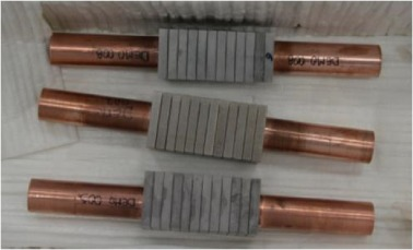
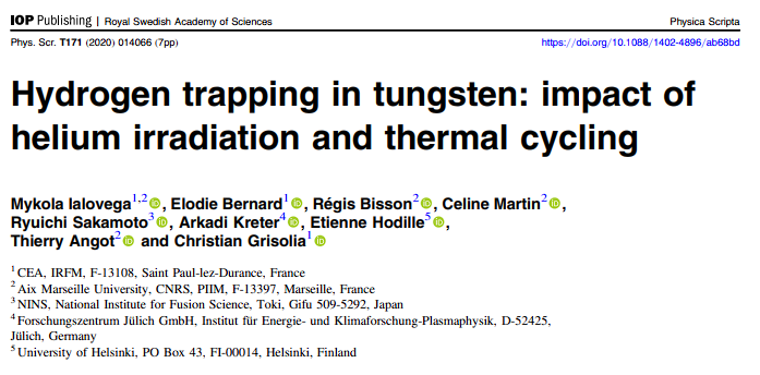
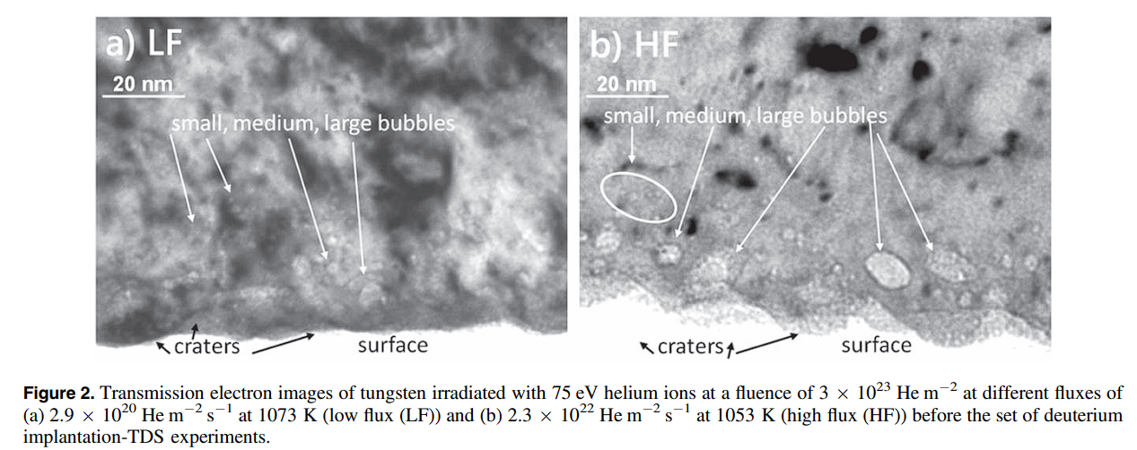
The bubble growth model was compared with experiments

Mykola Ialovega's PhD research

\(75 \ \mathrm{eV}\) He at \( 2.3 \times 10^ {22} \ \mathrm{m^{-2} \ s^{-1}}\) and \(1053 \ \mathrm{K} \) for \(13 \ \mathrm{s}\)
How to couple this to H transport?
Ialovega's experiment
He exposure
D exposure
Thermo-desorption
Repeat 5 times
W
Experimental conditions
Sample: \(100 \ \mathrm{\mu m} \) W
Pre-damage: \(75 \ \mathrm{eV}\) He at \( 2.3 \times 10^ {22} \ \mathrm{m^{-2} \ s^{-1}}\) and \(1053 \ \mathrm{K} \) for \(13 \ \mathrm{s}\)
Initial cleaning TDS after He implantation up to 870 K
D exposure: 250 eV at room temperature
Flux: \( 1.7 \times 10^ {16} \ \mathrm{m^{-2} \ s^{-1}}\)
Fluence: \( 4.5 \times 10^ {19} \ \mathrm{m^{-2}}\)
TDS temperature ramp: 1 K/s
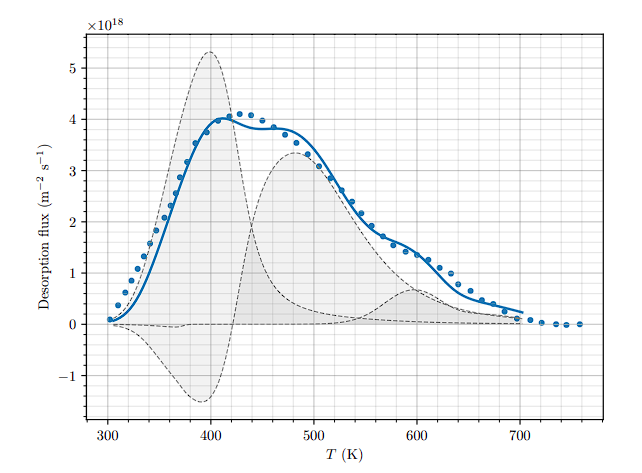
Ialovega's experiment
Ialovega's experiment

Lack of control experiment
❌No initial TDS
❌No cycling
❌Not performed at the time of the experiment
→ Can only be compared qualitatively!
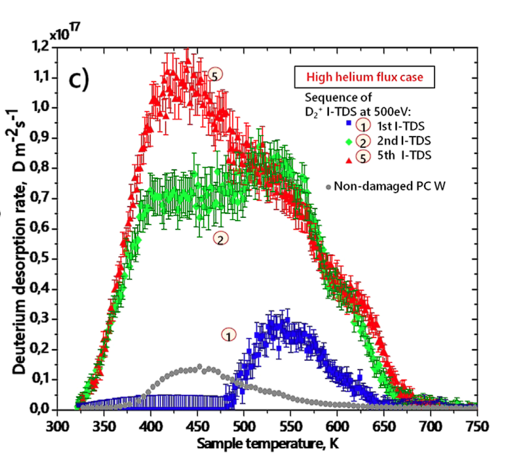
Ialovega's experiment

Ialovega's experiment


Ialovega's experiment
Correlation He release/D release
Hypotheses
- Helium doesn't desorb from bubbles
- Pre-existing defects exist (suggested by further analysis)
- Helium can saturate traps for Deuterium
\textcolor{#1f77b4}{n_b} = \textcolor{#ff7f0e}{c_b} \ f \ A(\langle r_b \rangle)
\mathrm{sites \, m^{-2}}
\mathrm{bubbles \, m^{-3}}
\mathrm{m^{2}}
surface coverage of trapping sites (tuning parameter)
f
\langle r_b \rangle = r_\mathrm{He_0 V_1} + \left( \frac{3}{4\pi} \frac{a_0^3}{2} \frac{\langle i_b \rangle}{4} \right) ^{1/3} - \left( \frac{3}{4\pi} \frac{a_0^3}{2} \right) ^{1/3}
bubbles radius
A = 4 \pi \langle r_b \rangle ^2
bubbles area

n_b
c_b
f = 3 \times 10 ^{18} \mathrm{m ^{-2}}
The He model was weakly coupled to FESTIM
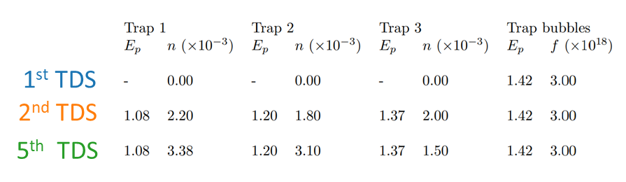
The model reproduced the experiment

Bubble-induced trap
- 4 traps including a bubble-induced trap
- TDS 1: density of available pre-existing traps is zero
- TDS 2-5: density of pre-existing traps \( \approx 2\times10^{-3}\ \mathrm{at.fr.}\)
- \( f \) is unchanged \( 3 \times 10^{18} \ \mathrm{m^{-2}}\)

Initial state

Pre-existing defects
He implantation
He implantation
1st D implantation
1st D implantation
1st TDS
He is removed from pre-existing defects
D is desorbed from bubbles
2nd D implantation
2nd D implantation
2nd D implantation
2nd TDS
D desorption from secondary defects
Repeat...
Impact on divertor inventory?
Divertor H inventory (g) at \( t = 10^7 \, \mathrm{s}\)
Increased trapping (bubbles)
Reduced trapping
(trap saturation)
Divertor inventory could be even lower
Main conclusions
- FESTIM was developed to assess T inventory in ITER plasma facing components and is now used for other applications (breeding blankets, experimental work...).
- Under conservative assumptions, the T inventory in the ITER divertor is below 1% of the in-vessel safety limit after 25 000 pulses.
- Results suggest that the presence of helium could reduce this inventory further by saturating traps.
Where to go from here?
- Validate the monoblock model with experimental data
- Retention in Be co-deposited layers will domitate the inventory
- Confirm/infirm our interpretation of the He-H interactions
- Investigate other in-vessel components like breeding blankets
k_\mathrm{burst} = e^{-x}
\frac{\partial c_b}{\partial t} = k_ {1,N}^+ c_1 c_N \\
\frac{\partial (\langle i_b \rangle c_b)}{\partial t} = (N+1)k_ {1,N}^+ c_1 c_N + \langle k_b^+ \rangle c_1 c_b \\ - \langle i_b \rangle k_\mathrm{burst} c_b
Adding bubble bursting


Thank you for your attention
Any questions?
Hydrogen transport in tokamaks
By Remi Delaporte-Mathurin
Hydrogen transport in tokamaks
This is the presentation I gave at my PhD defense on the 17th of October 2022


