


Sarah Dean PRO
asst prof in CS at Cornell
Fall 2025, Prof Sarah Dean
Text
How good are my prediction on data outside of the training set?
"What we do"
$$\theta_t = \arg\min_\theta \sum_{k=1}^t (\theta^\top x_k - y_k)^2 + \lambda\|\theta\|_2^2 $$
"Why we do it"
$$\theta_t = \arg\min_\theta \sum_{k=1}^t (\theta^\top x_k - y_k)^2 + \lambda\|\theta\|_2^2 $$
model
\(p_t:\mathcal X\to\mathcal Y\)
observation
prediction
\(x_t\)
Goal: cumulatively over time, predictions \(\hat y_t = p_t(x_t)\) are close to true \(y_t\)
accumulate
\(\{(x_t, y_t)\}\)
Online Learning
ex - rainfall prediction, online advertising, election forecasting, ...
Reference: Ch 1&2 of Shalev-Shwartz "Online Learning and Online Convex Optimization"
The regret of an algorithm which plays \((\hat y_t)_{t=1}^T\) in an environment playing \((x_t, y_t)_{t=1}^T\) is $$ R(T) = \sum_{t=1}^T \ell(y_t, \hat y_t) - \min_{p\in\mathcal P} \sum_{t=1}^T \ell(y_t, p(x_t)) $$
"best in hindsight"
often consider worst-case regret, i.e. \(\sup_{(x_t, y_t)_{t=1}^T} R(T)\)
"adversarial"
Online ERM aka "Follow the (Regularized) Leader"
$$\theta_t = \arg\min \sum_{k=1}^{t-1} \ell_k(\theta) + \lambda\|\theta\|_2^2$$
Online Gradient Descent
$$\theta_t = \theta_{t-1} - \alpha \nabla \ell_{t-1}(\theta_{t-1})$$
For simplicity, define \(\ell_t(\theta) = (x_t^\top \theta-y_t)^2\)
For differentiable and convex \(\ell:\mathcal \Theta\to\mathbb R\), $$\ell(\theta') \geq \ell(\theta) + \nabla \ell(\theta)^\top (\theta'-\theta)$$
Definition: \(\ell\) is \(L\)-Lipschitz continuous if there exists \(L\) so that for all \(\theta\in\Theta\) we have $$ \|\ell(\theta)-\ell(\theta')\|_2 \leq L\|\theta-\theta'\|_2 $$
A differentiable function \(\ell\) is \(L\)-Lipschitz if \(\|\nabla \ell(\theta)\|_2 \leq L\) for all \(\theta\in\Theta\).
Fact: The GD update is equivalent to $$\theta_t= \arg\min \nabla \ell_{t-1}(\theta_{t-1})^\top (\theta-\theta_{t-1}) +\frac{1}{2\alpha}\|\theta-\theta_{t-1}\|_2^2$$
Online Gradient Descent
$$\theta_t = \theta_{t-1} - \alpha \nabla \ell_{t-1}(\theta_{t-1})$$
because \( \theta_{t+1} = \arg\min\sum_{k=1}^{t} \nabla \ell_k(\theta_k)^\top\theta + \frac{1}{2\alpha}\|\theta\|_2^2\)
because by convexity, \(\ell_t(\theta) \geq \ell_t(\theta_t) + \nabla \ell_t(\theta_t)^\top (\theta-\theta_t)\)
For any fixed \(\theta\in\Theta\),
$$\textstyle \sum_{t=1}^T \ell_t(\theta_t)-\ell_t(\theta) \leq \sum_{t=1}^T \nabla \ell_t(\theta_t)^\top (\theta_t-\theta)$$
Can show by induction that for \(\theta_1=0\),
$$ \textstyle \sum_{t=1}^T \nabla \ell_t(\theta_t)^\top (\theta_t-\theta) \leq \frac{1}{2\alpha}\|\theta\|_2^2+ \sum_{t=1}^T \nabla \ell_t(\theta_t)^\top (\theta_t-\theta_{t+1})$$
\(=\frac{1}{2\alpha}\|\theta\|_2^2+ \sum_{t=1}^T \alpha\|\nabla \ell_t(\theta_t)\|_2^2\)
Putting it all together, $$ R(T) = \sum_{t=1}^T \ell_t(\theta_t)-\ell_t(\theta_\star) \leq \frac{1}{2\alpha}\|\theta_\star\|_2^2+ \alpha\sum_{t=1}^T L_t^2$$
because \(\ell_t\) is \(L_t\) Lipschitz
Finally, plug in \(\frac{1}{T}\sum_{t=1}^T L_t^2\leq L^2\),\(\|\theta_\star\|_2\leq B\), and set \(\alpha=\frac{L\sqrt{T}}{\sqrt{2}B}\).
Lemma (2.1, 2.3): For any fixed \(\theta\in\Theta\), under FTRL
$$ \sum_{t=1}^T \ell_t(\theta_t)-\ell_t(\theta) \leq \lambda\|\theta\|_2^2-\lambda\|\theta_1\|_2^2+ \sum_{t=1}^T \ell_t(\theta_t)-\ell_t(\theta_{t+1})$$
Lemma (2.10): For \(\ell_t\) convex and \(L_t\) Lipschitz,
$$ \ell_t(\theta_t)-\ell_t(\theta_{t+1}) \leq \frac{2L_t^2}{\lambda}$$
$$ R(T) = \sum_{t=1}^T \ell_t(\theta_t)-\ell_t(\theta_\star) \leq \lambda\|\theta_\star\| +2TL^2/\lambda$$
For linear functions, FTRL is exactly equivalent to OGD! In general, similar arguments.
Then we can write \(\hat\theta_t-\theta_\star\) when \(\lambda=0\)
Therefore, \((\hat\theta_t-\theta_\star)^\top x =\sum_{k=1}^t \varepsilon_k (V_t^{-1}x_k)^\top x\)
We have that \((\hat\theta_t-\theta_\star)^\top x =\sum_{k=1}^t \varepsilon_k (V_t^{-1}x_k)^\top x\) when \(\lambda=0\)
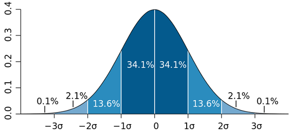
If \((\varepsilon_k)_{k\leq t}\) are Gaussian and independent from \((x_k)_{k\leq t}\), then this error is distributed as \(\mathcal N(0, \sigma^2\sum_{k=1}^t ((V_t^{-1}x_k)^\top x)^2)\)
With probability \(1-\delta\), we have \(|(\hat\theta_t-\theta_\star)^\top x| \leq \sigma\sqrt{2\log(2/\delta) }{\sqrt{x^\top V_t^{-1}x}}\)
z-score: w.p. \(1-\delta\), \(|u| \leq \sigma\sqrt{2\log(2/\delta)}\)
We have that \((\hat\theta_t-\theta_\star)^\top x =\sum_{k=1}^t \varepsilon_k (V_t^{-1}x_k)^\top x\) when \(\lambda=0\)
Gaussian case: \(1-\delta\) confidence interval is \(\theta_t^\top x\pm \sigma\sqrt{2\log(2/\delta) }{\sqrt{x^\top V_t^{-1}x}}\)
More generally, tail bounds of this form exist when:
\(\varepsilon_k\) is bounded (\(\beta\) has similar form) (Hoeffding's inequality)
\(\varepsilon_k\) is sub-Gaussian (\(\beta\) has similar form) (Markov's inequality)
\(\varepsilon_k\) has bounded variance (\(\beta\) scales with \(1/\delta\)) (Chebychev's inequality)
Reference: Ch 1&2 of Shalev-Shwartz "Online Learning and Online Convex Optimization", Ch 19-20 in Bandit Algorithms by Lattimore & Szepesvari
Next week: from prediction to action!
By Sarah Dean


