


Sarah Dean PRO
asst prof in CS at Cornell
June 2024
\(\to\)
historical interactions
probability of new interaction
1. Motivation: Implications for Personalization
2. Learning Dynamics from Bilinear Observations
inputs
outputs
time
1. Motivation: Implications for Personalization
\(u_t\)
\(y_t\)
Interests may be impacted by recommended content
preference state \(x_t\)
expressed preferences
recommended content
recommender policy
\(u_t\)
\(y_t = \langle x_t, u_t\rangle + w_t \)
Interests may be impacted by recommended content
expressed preferences
recommended content
recommender policy
underlies factorization-based methods
preference state \(x_t\)
\(u_t\)
\(y_t = \langle x_t, u_t\rangle + w_t \)
Interests may be impacted by recommended content
expressed preferences
recommended content
recommender policy
underlies factorization-based methods
state \(x_t\) updates to \(x_{t+1}\)
\(y_t = \langle x_t, u_t\rangle + v_t \)
\(x_{t+1} = f_t(x_t, u_t)\)
preferences \(x\in\mathcal X=\mathcal S^{d-1}\)
recommendations \(u_t\in\mathcal U\subseteq \mathcal S^{d-1}\)
initial preference
resulting preference
2. Biased assimilation
\(x_{t+1} \propto x_t + \eta_t\langle x_t, u_t\rangle u_t\)
When recommendations are made globally, the outcomes differ:
initial preference
resulting preference
1. Assimilation
\(x_{t+1} \propto x_t + \eta_t u_t\)
polarization (Hązła et al. 2019; Gaitonde et al. 2021)
homogenized preferences
Regardless of whether assimilation is biased,
Personalized fixed recommendation \(u_t=u\)
$$ x_t = \alpha_t x_0 + \beta_t u$$
positive and decreasing
increasing magnitude (same sign as \(\langle x_0, u\rangle\) if biased assimilation)
\(x_{t+1} \propto x_t + \eta_t\langle x_t, u_t\rangle u_t\)
\(x_{t+1} \propto x_t + \eta_t u_t\)
Regardless of whether assimilation is biased,
Implications [DM22]
It is not necessary to identify preferences to make high affinity recommendations
\(x_{t+1} \propto x_t + \eta_t\langle x_t, u_t\rangle u_t\)
\(x_{t+1} \propto x_t + \eta_t u_t\)
Regardless of whether assimilation is biased,
initial preference
resulting preference
Implications [DM22]
It is not necessary to identify preferences to make high affinity recommendations
Preferences "collapse" towards whatever users are often recommended
Non-manipulation (and other goals) can be achieved through randomization
\(x_{t+1} \propto x_t + \eta_t\langle x_t, u_t\rangle u_t\)
\(x_{t+1} \propto x_t + \eta_t u_t\)
Simple choice model: given a recommendation, a user
Preference dynamics lead to a new perspective on harm
Simple definition: harm caused by consumption of harmful content
\(\mathbb P\{\mathrm{click}\}\)
\(\circ\)
♫
𝅘𝅥
#
𝅘𝅥
♫
♫
𝅘𝅥𝅘𝅥
\(\circ\)
♫
𝅘𝅥
#
Without preference dynamics, harm minimizing policy is the engagement maximizing policy (excluding harmful items)
Recommendation: ♫
♫
𝅘𝅥𝅘𝅥
\(\circ\)
♫
𝅘𝅥
#
Recommendation: 𝅘𝅥
♫
𝅘𝅥
\(\circ\)
♫
𝅘𝅥
#
\(\mathbb P\{\mathrm{click}\}\)
\(\mathbb P \{\mathrm{click}\}\)
\(\circ\)
♫
𝅘𝅥
#
𝅘𝅥
♫
With preference dynamics, there may be downstream harm, even when no harmful content is recommended
Recommendation: ♫
♫
𝅘𝅥𝅘𝅥
\(\circ\)
♫
𝅘𝅥
#
Recommendation: 𝅘𝅥
♫
𝅘𝅥
\(\circ\)
♫
𝅘𝅥
#
\(\mathbb P\{\mathrm{click}\}\)
\(\mathbb P \{\mathrm{click}\}\)
\(\circ\)
♫
𝅘𝅥
#
𝅘𝅥
♫
With preference dynamics, there may be downstream harm, even when no harmful content is recommended
Recommendation: ♫
♫
𝅘𝅥𝅘𝅥
\(\circ\)
♫
𝅘𝅥
#
Recommendation: 𝅘𝅥
♫
𝅘𝅥
\(\circ\)
♫
𝅘𝅥
#
\(\mathbb P\{\mathrm{click}\}\)
\(\mathbb P \{\mathrm{click}\}\)
This motivates a new recommendation objective which takes into account the probability of future harm [CDEIKW24]
1. Motivation: Implications for Personalization
2. Learning Dynamics from Bilinear Observations
inputs
outputs
time
2. Learning Dynamics from Bilinear Observations
inputs
outputs
time
e.g. playlist attributes
e.g. listen time
inputs \(u_t\)
\( \)
outputs \(y_t\)
Input: data \((u_0,y_0,...,u_T,y_T)\), history length \(L\), state dim \(n\)
Step 1: Regression
$$\hat G = \arg\min_{G\in\mathbb R^{p\times pL}} \sum_{t=L}^T \big( y_t - u_t^\top \textstyle \sum_{k=1}^L G[k] u_{t-k} \big)^2 $$
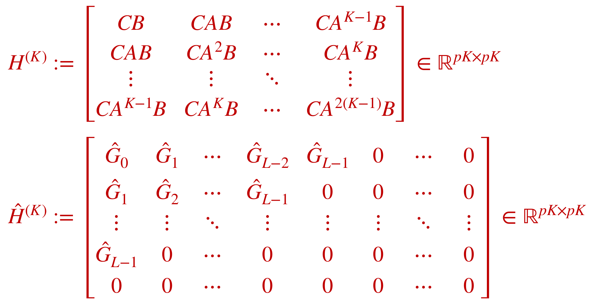
Step 2: Decomposition \(\hat A,\hat B,\hat C = \mathrm{HoKalman}(\hat G, n)\)
\(t\)
\(L\)
\(\underbrace{\qquad\qquad}\)
inputs
outputs
time
$$\hat G = \arg\min_{G\in\mathbb R^{p\times pL}} \sum_{t=L}^T \big( y_t - u_t^\top \textstyle \sum_{k=1}^L G[k] u_{t-k} \big)^2 $$
\(t\)
\(L\)
\(\underbrace{\qquad\qquad}\)
\(\bar u_{t-1}^\top \otimes u_t^\top \mathrm{vec}(G) \)
inputs
outputs
time
$$\hat G = \arg\min_{G\in\mathbb R^{p\times pL}} \sum_{t=L}^T \big( y_t - u_t^\top \textstyle \sum_{k=1}^L G[k] u_{t-k} \big)^2 $$
\(\bar u_{t-1}^\top \otimes u_t^\top \mathrm{vec}(G) \)
\(*\)
\(=\)
\(\underbrace{\qquad\qquad}\)
\(\underbrace{\qquad\qquad}\)
\(\underbrace{\qquad\qquad}\)
\(\underbrace{\qquad\qquad\qquad}\)
\(t\)
\(L\)
\(\underbrace{\qquad\qquad}\)
inputs
outputs
time
Assumptions:
With probability at least \(1-\delta\), $$\epsilon_G=\|G-\hat G\|_{\tilde U^\top \tilde U} \lesssim \sqrt{ \frac{p^2 L}{\delta} \cdot c_{\mathrm{stability,noise}} }+ \rho(A)^L\sqrt{T} c_{\mathrm{stability}}$$
Assumptions:
Suppose \(L\) is sufficiently large. Then, there exists a nonsingular matrix \(S\) (i.e. a similarity transform) such that
\(\|A-S\hat AS^{-1}\|_{F}\)
\(\| B-S\hat B\|_{F}\)
\(\| C-\hat CS^{-1}\|_{F} \)
$$\lesssim c_{\mathrm{contr,obs,dim}} \frac{\|G-\hat G\|_{F}}{\sqrt{\sigma_{\min}(\tilde U^\top \tilde U)}} $$
\(\underbrace{\qquad\qquad}\)
Assumptions:
With high probabilty, $$\mathrm{est.~errors} \lesssim \sqrt{ \frac{\mathsf{poly}(\mathrm{dimension})}{\sigma_{\min}(\tilde U^\top \tilde U)}}$$
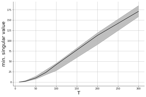
When \(u_t\) are chosen i.i.d. and sub-Gaussian and \(T\) is large enough, whp $$\sigma_{\min}({\tilde U^\top \tilde U} )\gtrsim T$$
For i.i.d. and sub-Gaussian inputs, whp $$\mathrm{est.~errors} \lesssim \sqrt{ \frac{\mathsf{poly}(\mathrm{dim.})}{T}}$$
How large does \(T\) need to be to guarantee bounded estimation error?
\(*\)
\(=\)
formal analysis involves the structured random matrix \(\tilde U\)
inputs
outputs
time
Other References
more details on affinity maximization, preference stationarity, and mode collapse
(Oymak & Ozay, 2019)
$$\hat G = \arg\min_{G\in\mathbb R^{p\times pL}} \sum_{t=L}^T \big( y_t - \bar u_{t-1}^\top \otimes u_t^\top \mathrm{vec}(G) \big)^2 $$
Set of equivalent state space representations for all invertible and square \(M\)
\(s_{t+1} = As_t + Bw_t\)
\(y_t = Cs_t+v_t\)
\(\tilde s_{t+1} = \tilde A\tilde s_t + \tilde B w_t\)
\(y_t = \tilde C\tilde s_t+v_t\)
\(\tilde s = M^{-1}s\)
\(\tilde A = M^{-1}AM\)
\(\tilde B = M^{-1}B\)
\(\tilde C = CM\)
\( s = M\tilde s\)
\( A = M\tilde AM^{-1}\)
\( B = M\tilde B\)
\(C = \tilde CM^{-1}\)
\(y_t\)
\(A\)
\(s\)
\(w_t\)
\(v_t\)
\(C\)
\(B\)
\(y_t\)
\(\tilde A\)
\(s\)
\(w_t\)
\(v_t\)
\(\tilde C\)
\(\tilde B\)
By Sarah Dean


