Learning Models of Dynamical Systems from Finite Observations

Sarah Dean, Cornell University

SYSID, July 2024

Large-scale automated systems

enabled by machine learning

$\to$

historical interactions

probability of new interaction

Feedback arises when actions impact the world

Training data is correlated due to dynamics and feedback

Outline

1. Modern Finite-Sample Perspectives

2. Towards SysId for Personalization

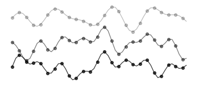
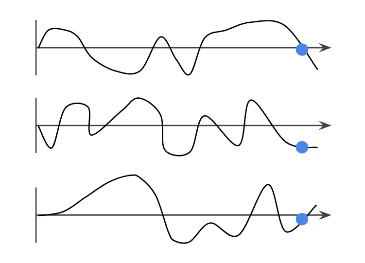
inputs

outputs

time

Outline

1. Modern Finite-Sample Perspectives

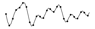
inputs

outputs

time

i) Overview

ii) LQR

iii) Extensions

Traditional perspective: asymptotic statistics & consistency
90s-00s: beginnings of non-asymptotic analysis
Last 5-10 years: modern analyses with a learning theory perspective

Finite-sample Perspectives on SysId

Statistical Learning Theory for Control: A Finite Sample Perspective

Anastasios Tsiamis, Ingvar Ziemann, Nikolai Matni, George J. Pappas IEEE Control Systems Magazine

Sample Complexity: How much data is necessary to learn a system?

Given error $\epsilon$ and failure probability $\delta$, how many samples are necessary to ensure $\mathbb P(\text{estimation err.}\geq \epsilon)\leq\delta$?

Sample Complexity of LQR

Work with Horia Mania, Nikolai Matni, Ben Recht, and Stephen Tu in 2017

Motivation: foundation for understanding RL & ML-enabled control

building on the adaptive perspective by Abbasi-Yadkori & Szepesvári (2011)

Classic RL setting: discrete problems and inspired by games

RL techniques applied to continuous systems interacting with the physical world

Linear Quadratic Regulator

Simplest problem: linear dynamics, quadratic cost, Gaussian process noise

minimize $\mathbb{E}\left[ \displaystyle\lim_{T\to\infty}\frac{1}{T}\sum_{t=0}^T x_t^\top Q x_t + u_t^\top R u_t\right]$

s.t. $x_{t+1} = Ax_t+Bu_t+w_t$

$u_t = \underbrace{-(R+B^\top P B)^{-1} B^\top P A}_{K_\star}x_t$

where $P=\text{DARE}(A,B,Q,R)$ also defines the value function $V(x) = x^\top P x$

Static feedback controller is optimal and can be computed in closed-form:

Sample Complexity Problem

How many observations are necessary to control unknown system?

Main Result (Informal):

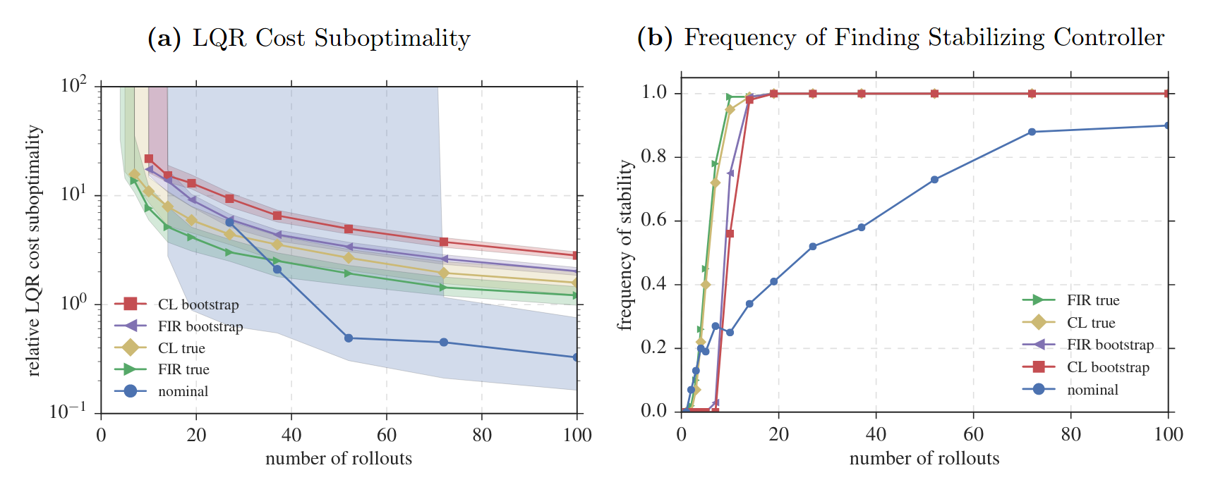
As long as $N$ is large enough, then with probability at least $1-\delta$,
$\mathrm{rel.~error~of}~\widehat{\mathbf K}\lesssim \frac{\mathrm{size~of~noise}}{\mathrm{size~of~excitation}} \sqrt{\frac{\mathrm{dimension}}{N} \log(1/\delta)} \cdot\mathrm{robustness~of~}K_\star$

excitation

$(A_\star, B_\star)$

$N$ observations

Approach: Coarse-ID Control

1. Collect $N$ observations and estimate $\widehat A,\widehat B$ and confidence intervals

2. Use estimates to synthesize robust controller $\widehat{\mathbf{K}}$

$(A_\star, B_\star)$

$\widehat{\mathbf{K}}$

$(A_\star, B_\star)$

$\|\hat A-A_\star\|\leq \epsilon_A$

$\|\hat B-B_\star\|\leq \epsilon_B$

Main Control Result (Informal):

rel. error of $\widehat{\mathbf K}\lesssim (\epsilon_A+\epsilon_B\|K_\star\|) \|\mathscr{R}_{A_\star+B_\star K_\star}\|_{\mathcal H_\infty}$

robustness of $K_\star$

System Identification

Least squares estimate: $(\widehat A, \widehat B) \in \arg\min \sum_{\ell=1}^N \|Ax_{T}^{(\ell)} +B u_{T}^{(\ell)} - x_{T+1}^{(\ell)}\|^2 $

Learning Result:

As long as $N\gtrsim n+p+\log(1/\delta)$, then with probability at least $1-\delta$,

$\|\widehat A - A_\star\| \lesssim \frac{\sigma_w}{\sqrt{\lambda_{\min}(\sigma_u^2 G_T G_T^\top + \sigma_w^2 F_T F_T^\top )}} \sqrt{\frac{n+p }{N} \log(1/\delta)} $, $\|\widehat B - B_\star\| \lesssim \frac{\sigma_w}{\sigma_u} \sqrt{\frac{n+p }{N} \log(1/\delta)} $

with controllability Grammians defined as

$G_T = \begin{bmatrix}A_\star^{T-1}B_\star&A_\star^{T-2}B_\star&\dots&B_\star\end{bmatrix} \qquad F_T = \begin{bmatrix}A_\star^{T-1}&A_\star^{T-2}&\dots&I\end{bmatrix}$

$(A_\star, B_\star)$

Excitation

$u_t^{(\ell)} \sim \mathcal{N}(0, \sigma_u^2)$

Observe states $\{x_t^{(\ell)}\}$

I.i.d. Random Matrix Analysis

have independent Gaussian entries

$\begin{bmatrix} x_{T}^{(\ell)} \\u_{T}^{(\ell)} \end{bmatrix} \sim \mathcal{N}\left(0, \begin{bmatrix}\sigma_u^2 G_TG_T^\top + \sigma_w^2 F_TF_T^\top &\\ & \sigma_u^2 I\end{bmatrix}\right)$

$w_t^{(\ell)} \sim \mathcal{N}\left(0, \sigma_w^2\right)$

The least-squares estimate is

$\arg \min \|Z_N \begin{bmatrix} A & B\end{bmatrix} ^\top - X_N\|^2_F = (Z_N^\top Z_N)^\dagger Z_N^\top X_N$

$= \begin{bmatrix} A_\star & B_\star \end{bmatrix} ^\top + (Z_N^\top Z_N)^\dagger Z_N^\top W_N$

Data and noise matrices

$X_N = \begin{bmatrix} x_{T+1}^{(1)} & \dots & x_{T+1}^{(N)} \end{bmatrix}^\top$

$Z_N = \begin{bmatrix} x_{T}^{(1)} & \dots & x_{T}^{(N)} \\u_{T}^{(1)} & \dots & u_{T}^{(N)} \end{bmatrix}^\top$

$W_N = \begin{bmatrix} w_{T}^{(1)} & \dots & w_{T}^{(N)} \end{bmatrix}^\top $

lower bound minimum singular value,

or compute data-dependent bound

upper bound inner products

Single Trajectory Identification

Multi-trajectory setting (previous slide): excitable & less stable systems are easier to learn
Classic mixing time analysis: more stable systems are easier to learn because data is closer to being independent
Followup work by Simchowitz et al. (2018) on Learning without Mixing show that strict stability is not required!$$\Big\|\begin{bmatrix} \widehat A - A_\star \\ \widehat B - B_\star\end{bmatrix}\Big\| \lesssim \frac{\sigma_w}{C_u \sigma_u}\sqrt{\frac{n+p }{T} \log(d/\delta)} $$

$(A_\star, B_\star)$

Extension: Online Control

1. Excite system for $N$ steps and estimate $\widehat A,\widehat B$

2. Run controller $\widehat{\mathbf{K}}$ for remaining time $T-N$

$(A_\star, B_\star)$

$\widehat{\mathbf{K}}$

$(A_\star, B_\star)$

Exploration vs. Excitation
Average sub-optimality of Robust Adaptive Control is $\mathcal O(T^{-1/3})$ [DMMRT18]
For Certainty Equivalent Adaptive Control, $\mathcal O(T^{-1/2})$ (Mania et al., 2019)

Further Extensions

Safety constraints [DTMR19]
- Robust controller compensates for bounded exploration noise to keep system safe during exploration
Perception-based control [DMRY20,DR21]
- Nonlinear observation model with $y_t = g(x_t)$ for invertible $g$
Any many others! Non-stochastic control, partial observation & LQG, set membership identification

Outline

1. Modern Finite-Sample Perspectives

2. Towards SysId for Personalization

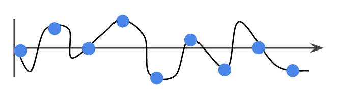
inputs

outputs

time

Outline

2. Towards SysId for Personalization

i) Personalization

ii) Preference Dynamics

iii) Identification

iv) Open Questions

Setting: Personalization

$u_t$

$y_t$

Classically studied as an online decision problem (e.g. multi-armed bandits)

unknown preference

expressed preferences

Setting: Personalization

$u_t$

unknown preference $x$

expressed preferences

Setting: Preference Dynamics

$u_t$

However, interests may be impacted by recommended content

preference state $x_t$

expressed preferences

Example: Preference Dynamics

Implications for personalization [DM22]

It is not necessary to estimate preferences to make "good" recommendations
Preferences "collapse" towards whatever users are often recommended
Non-manipulation (and other goals) can be achieved through randomization
Even if harmful content is never recommended, can cause harm through preference shifts [CDEIKW24]

initial preference
resulting preference
recommendation

Problem Setting: Identification

Unknown dynamics and measurement functions
Observed trajectory of inputs $u\in\mathbb R^p$ and outputs $y\in\mathbb R$ $$u_0,y_0,u_1,y_1,...,u_T,y_T$$
Goal: identify dynamics and measurement models from data
Setting: linear/bilinear with $A\in\mathbb R^{n\times n}$, $B\in\mathbb R^{n\times p}$, $C\in\mathbb R^{p\times n}$ $$x_{t+1} = Ax_t + Bu_t + w_t\\ y_t = u_t^\top Cx_t + v_t$$

e.g. playlist attributes

e.g. listen time

inputs $u_t$

outputs $y_t$

Identification Algorithm

Input: data $(u_0,y_0,...,u_T,y_T)$, history length $L$, state dim $n$

Step 1: Regression

$$\hat G = \arg\min_{G\in\mathbb R^{p\times pL}} \sum_{t=L}^T \big( y_t - u_t^\top \textstyle \sum_{k=1}^L G[k] u_{t-k} \big)^2 $$

Step 2: Decomposition $\hat A,\hat B,\hat C = \mathrm{HoKalman}(\hat G, n)$

$t$

$L$

$\underbrace{\qquad\qquad}$

inputs

outputs

time

Yahya Sattar

$~$

Estimation Errors

$$\hat G = \arg\min_{G\in\mathbb R^{p\times pL}} \sum_{t=L}^T \big( y_t - u_t^\top \textstyle \sum_{k=1}^L G[k] u_{t-k} \big)^2 $$

(Biased) estimate of Markov parameters $$ G =\begin{bmatrix} C B & CA B & \dots & CA^{L-1} B \end{bmatrix} $$
Regress $y_t$ against $$ \underbrace{ \begin{bmatrix} u_{t-1}^\top & ... & u_{t-L}^\top \end{bmatrix}}_{\bar u_{t-1}^\top } \otimes u_t^\top $$
Data matrix: circulant-like structure $$Z = \begin{bmatrix}\bar u_{L-1}^\top \otimes u_L^\top \\ \vdots \\ \bar u_{T-1}^\top \otimes u_T^\top\end{bmatrix} $$

$t$

$L$

$\underbrace{\qquad\qquad}$

$\bar u_{t-1}^\top \otimes u_t^\top \mathrm{vec}(G) $

inputs

outputs

time

$*$

$=$

$\underbrace{\qquad\qquad}$

$\underbrace{\qquad\qquad\qquad}$

$$Z = \begin{bmatrix}\bar u_{L-1}^\top \otimes u_L^\top \\ \vdots \\ \bar u_{T-1}^\top \otimes u_T^\top\end{bmatrix} $$

Main Results

Assumptions:

Process and measurement noise $w_t,v_t$ are i.i.d., zero mean, and have bounded second moments
Inputs $u_t$ are bounded
The dynamics are strictly stable, i.e. $\rho(A)<1$

Informal Theorem (Markov parameter estimation)

With probability at least $1-\delta$, $$\|G-\hat G\|_{Z^\top Z} \lesssim \sqrt{ \frac{p^2 L}{\delta} \cdot c_{\mathrm{stability,noise}} }+ \rho(A)^L\sqrt{T} c_{\mathrm{stability}}$$

Main Results

Assumptions:

Process and measurement noise $w_t,v_t$ are i.i.d., zero mean, and have bounded second moments
Inputs $u_t$ are bounded
The dynamics are strictly stable, i.e. $\rho(A)<1$
(For state space recovery: $(A,B,C)$ are observable, controllable)

Informal Summary Theorem

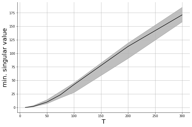
With high probabilty, $$\mathrm{est.~errors} \lesssim \sqrt{ \frac{\mathsf{poly}(\mathrm{dimension})}{\sigma_{\min}(Z^\top Z)}}$$

Open Q: Sample Complexity

Informal Conjecture

When $u_t$ are chosen i.i.d. and sub-Gaussian and $T$ is large enough, whp $$\sigma_{\min}({Z^\top Z} )\gtrsim T$$

Informal Corollary

For i.i.d. and sub-Gaussian inputs, whp $$\mathrm{est.~errors} \lesssim \sqrt{ \frac{\mathsf{poly}(\mathrm{dim.})}{T}}$$

How large does $T$ need to be to guarantee bounded estimation error?

$*$

$=$

formal analysis involves the structured random matrix $Z$

$$ = \begin{bmatrix}\bar u_{L-1}^\top \otimes u_L^\top \\ \vdots \\ \bar u_{T-1}^\top \otimes u_T^\top\end{bmatrix} $$

Open Qs:

Sample complexity (data independent)
- Idea: random design
- Challenge: dependent matrix entries
Relax assumption on stability of $A$
- Idea: regress $y_t$ against $u_{0:t},y_{0:t-1}$
- Challenge: sample complexity of partially observed bilinear sysid
Effect on preference prediction?
- Idea: Kalman filter (certainty equivalent vs. robust)
Effect on optimal recommendation?
- Challenge: difficult optimal control problem

Conclusion

1. Modern Finite-Sample Perspectives

2. Towards SysId for Personalization

Questions about decision-making from the learning theory perspective motivate new system identification results

inputs

outputs

time

On the sample complexity of the linear quadratic regulator in Foundations of Computational Mathematics (2019) with Horia Mania, Nikolai Matni, Ben Recht, Stephen Tu
Learning Linear Dynamics from Bilinear Observations (in preparation) with Yahya Sattar

Thanks! Questions?

Regret bounds for robust adaptive control of the linear quadratic regulator at NeuRIPS18 () with Mania, Matni, Recht, Tu
Preference Dynamics Under Personalized Recommendations at EC22 (arxiv:2205.13026) with Jamie Morgenstern
Harm Mitigation in Recommender Systems under User Preference Dynamics at KDD24 (arxiv:2406.09882) with Chee, Ernala, Ioannidis, Kalyanaraman, Weinsberg

Abbasi-Yadkori, Szepesvári. "Regret bounds for the adaptive control of linear quadratic systems." COLT, 2011.
Anderson, Doyle, Low, Matni. "System level synthesis." Annual Reviews in Control (2019).
Dean, Matni, Recht, Ya. "Robust Guarantees for Perception-Based Control." L4DC, 2020.
Dean, Tu, Matni, Recht. "Safely learning to control the constrained linear quadratic regulator." ACC, 2019
Gaitonde, Kleinberg, Tardos, 2021. Polarization in geometric opinion dynamics. EC.
Hązła, Jin, Mossel, Ramnarayan, 2019. A geometric model of opinion polarization. Mathematics of Operations Research.
Mania, Tu, Recht. "Certainty Equivalence is Efficient for Linear Quadratic Control." NeuRIPS, 2019.
Omyak & Ozay, 2019. Non-asymptotic Identification of LTI Systems from a Single Trajectory. ACC.
Simchowitz, Mania, Tu, Jordan, Recht. "Learning without mixing: Towards a sharp analysis of linear system identification." COLT, 2018.

Main LQR Result

As long as $N\gtrsim (n+p)\sigma_w^2\|\mathscr R_{A_\star+B_\star K_\star}\|_{\mathcal H_\infty}(1/\lambda_G + \|K_\star\|^2/\sigma_u^2)\log(1/\delta)$, then for robustly synthesized $\widehat{\mathbf{K}}$, with probability at least $1-\delta$,

rel. error of $\widehat{\mathbf K}$ $\lesssim \sigma_w (\frac{1}{\sqrt{\lambda_G}} + \frac{\|K_\star\|}{\sigma_u}) \|\mathscr{R}_{A_\star+B_\star K_\star}\|_{\mathcal H_\infty} \sqrt{\frac{n+p }{T} \log(1/\delta)}$

robustness of optimal closed-loop

excitability of system

optimal controller gain

vs.

Experimental Results

more details on affinity maximization, preference stationarity, and mode collapse

Proof Sketch

$$\hat G = \arg\min_{G\in\mathbb R^{p\times pL}} \sum_{t=L}^T \big( y_t - \bar u_{t-1}^\top \otimes u_t^\top \mathrm{vec}(G) \big)^2 $$

Claim: this is a biased estimate of Markov parameters $$ G_\star =\begin{bmatrix} C B & CA B & \dots & CA^{L-1} B \end{bmatrix} $$
- Observe that $x_t = \sum_{k=1}^L CA^{k-1} B (u_{t-k} + w_{t-k}) + A^L x_{t-L}$
- Hence, $y_t= \bar u_{t-1}^\top \otimes u_t^\top \mathrm{vec}(G_\star) +u_t^\top \textstyle \sum_{k=1}^L CA^{k-1} w_{t-k} + u_t CA^L x_{t-L} + v_t $
Least squares: for $y_t = z_t^\top \theta + n_t$, the estimate $\hat\theta=\arg \min\sum_t (z_t^\top \theta - y_t)^2$ $$= \textstyle\arg \min \|Z \theta - Y\|^2_2 = (Z^\top Z)^\dagger Z^\top Y= \theta_\star + (Z^\top Z)^\dagger Z^\top N$$
Estimation errors are therefore $\|G_\star -\hat G\|_{\tilde U^\top\tilde U} = \|\tilde U^\top N\| $

Main Results

Assumptions:

Process and measurement noise $w_t,v_t$ are i.i.d., zero mean, and have bounded second moments
Inputs $u_t$ are bounded
The dynamics $(A,B,C)$ are observable, controllable, and strictly stable, i.e. $\rho(A)<1$

Informal Theorem (system identification)

Suppose $L$ is sufficiently large. Then, there exists a nonsingular matrix $S$ (i.e. a similarity transform) such that

$\|A-S\hat AS^{-1}\|_{Z^\top Z}$

$\| B-S\hat B\|_{Z^\top Z}$

$\| C-\hat CS^{-1}\|_{Z^\top Z} $

$$\lesssim c_{\mathrm{contr,obs,dim}} \|G-\hat G\|_{Z^\top Z} $$

$\underbrace{\qquad\qquad}$

Learning Models of Dynamical Systems from Finite Observations

By Sarah Dean

Learning Models of Dynamical Systems from Finite Observations

Sarah Dean PRO

asst prof in CS at Cornell

sdean.website

Learning Models of Dynamical Systems from Finite Observations

Sarah Dean, Cornell University

Large-scale automated systems

enabled by machine learning

Feedback arises when actions impact the world

Training data is correlated due to dynamics and feedback

Outline

Outline

i) Overview

ii) LQR

iii) Extensions

Finite-sample Perspectives on SysId

Sample Complexity of LQR

Linear Quadratic Regulator

Sample Complexity Problem

Main Result (Informal):

Approach: Coarse-ID Control

System Identification

Learning Result:

I.i.d. Random Matrix Analysis

Single Trajectory Identification

Extension: Online Control

Further Extensions

Outline

Outline

i) Personalization

ii) Preference Dynamics

iii) Identification

iv) Open Questions

Setting: Personalization

Setting: Personalization

Setting: Preference Dynamics

Example: Preference Dynamics

Problem Setting: Identification

Identification Algorithm

Estimation Errors

Main Results

Informal Theorem (Markov parameter estimation)

Main Results

Informal Summary Theorem

Open Q: Sample Complexity

Informal Conjecture

Informal Corollary

Open Qs:

Conclusion

Thanks! Questions?

Main LQR Result

Experimental Results

Proof Sketch

Main Results

Informal Theorem (system identification)

Learning Models of Dynamical Systems from Finite Observations

More from Sarah Dean