Sarah Dean PRO
asst prof in CS at Cornell
(down arrow to see handout slides)
$$ \mathbf{X}\mathbf{X}^\top\mathbf{w} = \mathbf{X}\mathbf{y}^\top $$
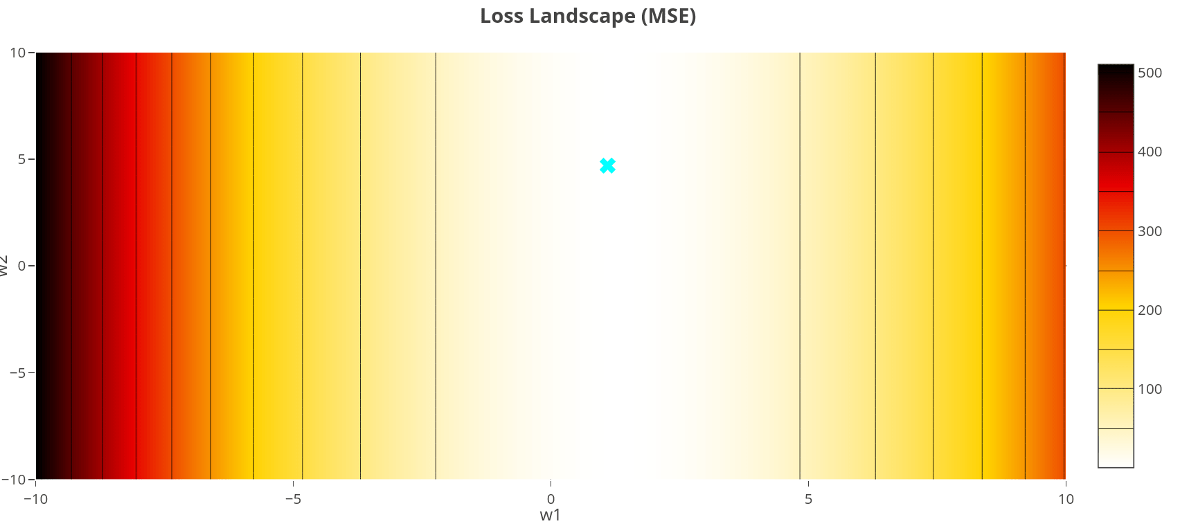
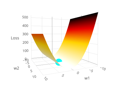
\(\lambda=0\)
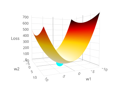
\(\lambda=1\)
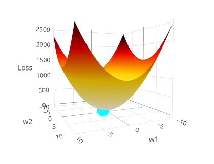
\(\lambda=10\)
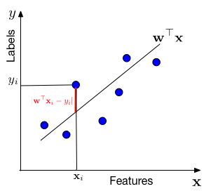
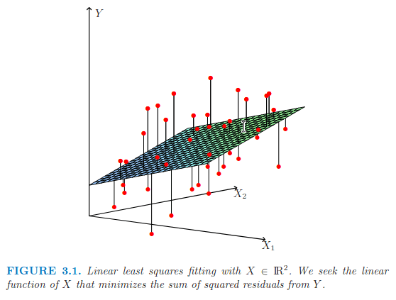
Data & Model Assumption: Same setup \(y_i = \mathbf{w}^\top\mathbf{x}_i + \epsilon_i\), but now we also assume weights are small.
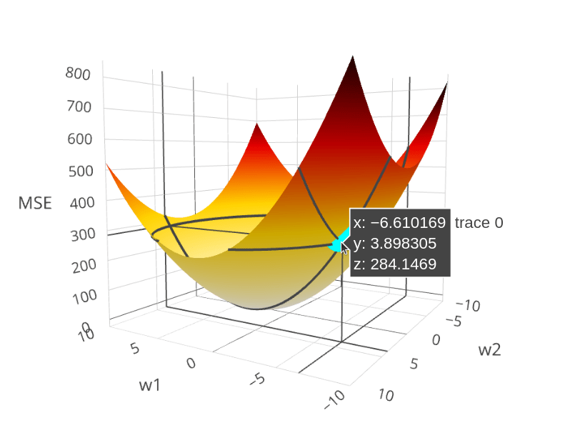
Ridge Objective: minimize squared errors plus a penalty on weight size, where \(\lambda > 0\): $$ \min_{\mathbf{w}} \frac{1}{n}\sum_{i=1}^n (\mathbf{x}_i^\top\mathbf{w} - y_i)^2 + \lambda\|\mathbf{w}\|_2^2 $$
MAP connection: This objective is equivalent to MAP estimation, maximizing \(P(\mathbf{w}|D) \propto P(D|\mathbf{w})P(\mathbf{w})\), with the Gaussian prior: $$ P(\mathbf{w}) = \frac{1}{\sqrt{2\pi\tau^2}}e^{-\frac{\mathbf{w}^\top\mathbf{w}}{2\tau^2}} \quad \Rightarrow \quad \lambda = \frac{\sigma^2}{n\tau^2} $$
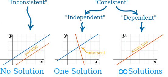
Closed-form solution: Set gradient to zero and solve (always unique): $$ \mathbf{w}^* = (\mathbf{X}\mathbf{X}^\top + n\lambda\mathbf{I})^{-1}\mathbf{X}\mathbf{y}^\top $$
Ordinary Least Squares (unregularized):
Ridge Regression (regularized):
By Sarah Dean


