
Project Management & Communication
Sebastian Hörl
28 January 2022
Université Gustave Eiffel
This part of the course
- Today + next week: Lecture
- Basic concepts in transport planing
- Four-step models vs. activity-based models
- Coming sessions: Project work
- 18 February, 14:00 - 16:00
- 11 March, 14:00 - 17:00
- 25 March, 14:00 - 17:00
- Assessment
- Final presentation (25 March)
- Short report (until 8 April)
Today
- Introduction to transport planning
- Four-step models
- Activity-base models
- Agent-based models
- Details on the course project
- Four different groups
- Interaction and assessment criteria
- Time plan and definition of groups
Transport planning: Overview
- Goals
- Cost-benefit analysis
- Assessment of alternatives
- Prediction
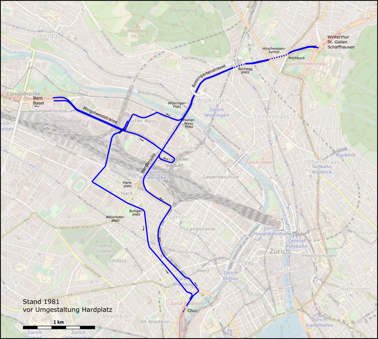
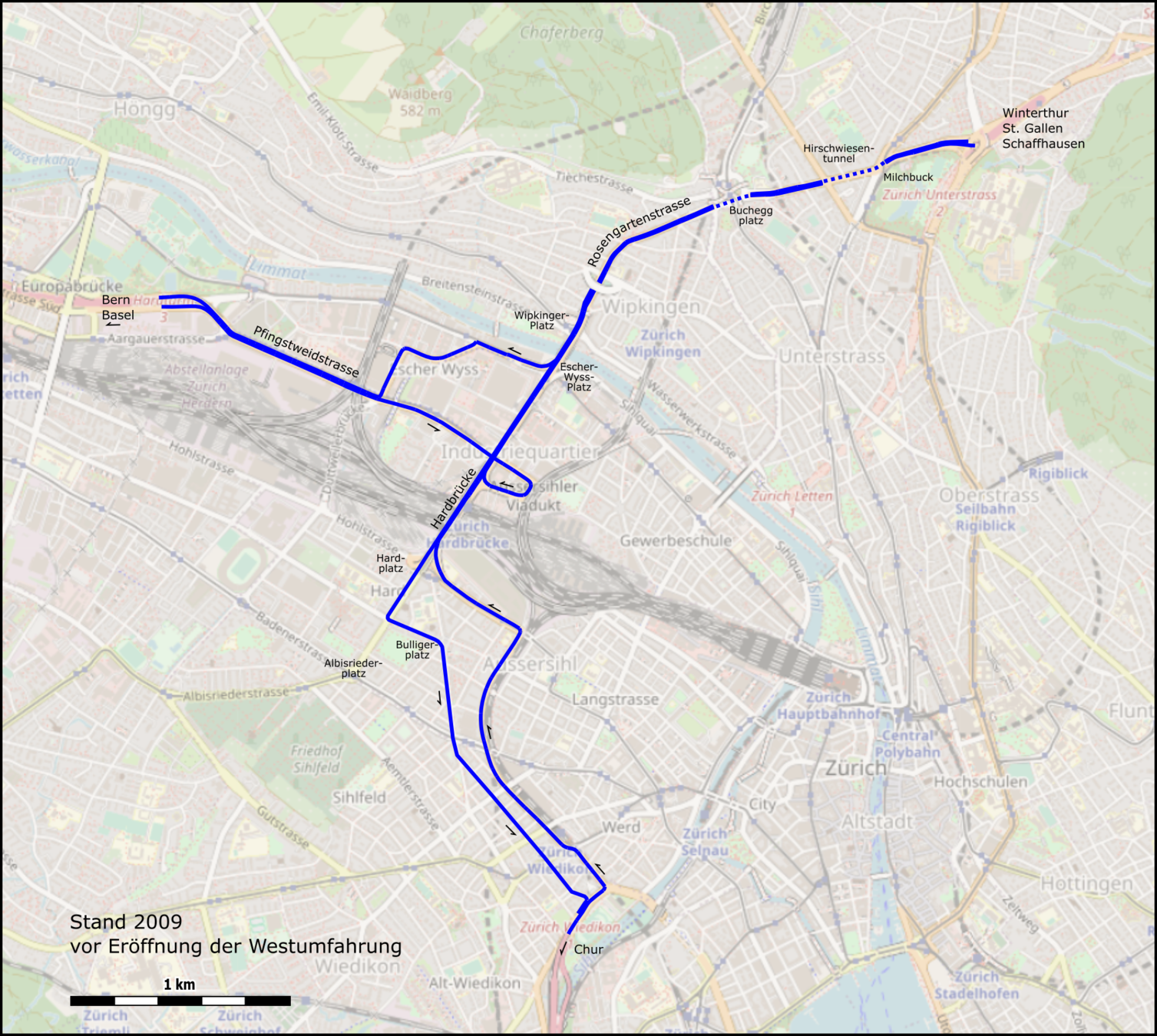
Sources: https://de.wikipedia.org/wiki/Westtangente_Z%C3%BCrich, openstreetmap.org
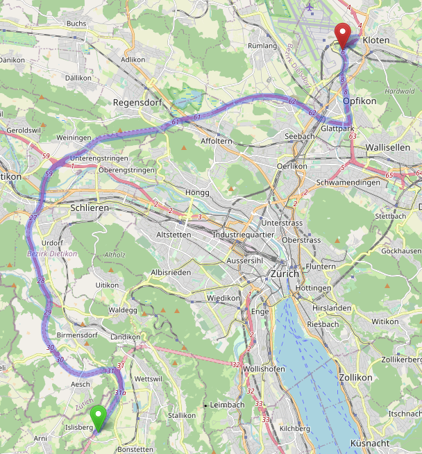
Transport planning: Overview
- Goals
- Cost-benefit analysis
- Assessment of alternatives
- Prediction
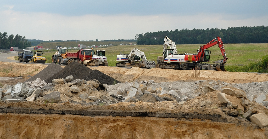
- Use cases
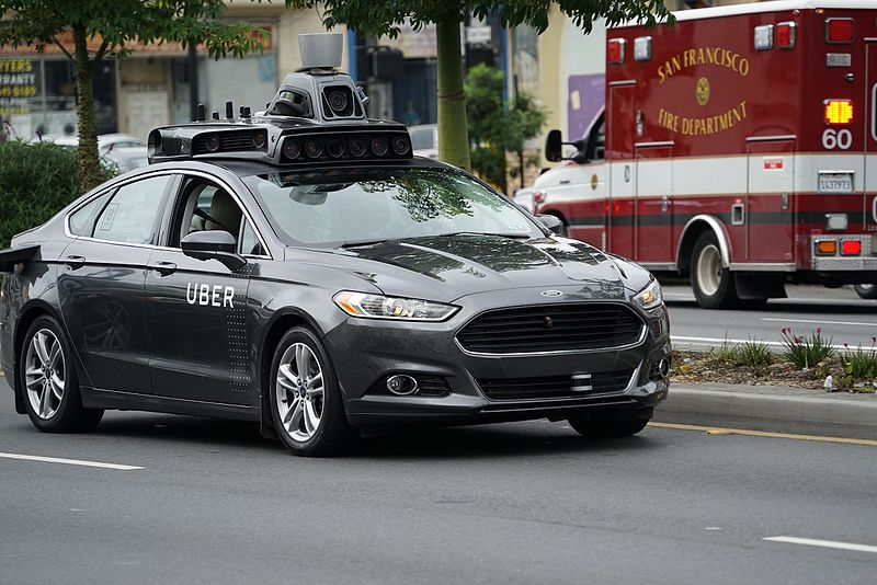
- Traditionally: Infrastructure
- Today: Increasingly digital technology
Sources:
https://en.wikipedia.org/wiki/File:Highway_8_widening.png
https://commons.wikimedia.org/wiki/File:Self_driving_Uber_prototype_in_San_Francisco.jpg
Transport planning: Overview
- Traditional approaches
- High aggregation
- Movements are flows
- Locations are zones
- Specific times of the day
- Today's approaches
- Individual entities
- Movements are detailed in time and space
- Whole daily analysis possible
Four-step models
Activity-based models
Four-step model: Overview
Generation
Distribution
Mode choice
Assignment
- Four steps making use of different data sources
- From static to more dynamic mobility decisions
- Multiple possible feedback loops (most common example here)
Four-step model: Overview
Generation
Distribution
Mode choice
Assignment
- Where do trips appear?
- What is the destination of the trips?
- What transport mode is used?
- What congestion is caused?
Four-step model: Overview
Generation
Distribution
Mode choice
Assignment
Travel demand
Travel supply
- Characterizes the need for mobility in the population for economic activity, leisure, ...
- Means that allow for mobility
- Road infrastructure, rail network, ...
Four-step model: Overview
Generation
Distribution
Mode choice
Assignment
Travel demand
Travel supply
- Characterizes the need for mobility in the population for economic activity, leisure, ...
- Means that allow for mobility
- Road infrastructure, rail network, ...
Equilibrium
- Given limited capacity,
how is the system used?
Four-step model: Trip generation
-
Goal: Define statistically where trips starts, i.e. where they are "generated" or produced
- Focus on peak hours in 4S, e.g. morning peak and focus on commuting activity
- Either making use of direct data (e.g. from surveys) or based on population data, land use information, ...
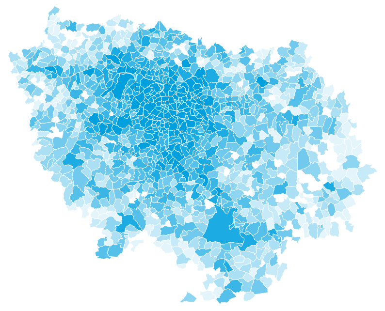
Number of inabitants in Île-de-France
Four-step model: Trip generation
- May be per homogeneous user group, e.g.
- Single-person households
- Multi-persons households
without children - Multi-person households
with children -
Households with retired persons
- Possible to use statistical models
O_{s,g} = f(X_s)
Generated trips
in zone s in group g
Trip generation model
Model inputs
Four-step model: Trip generation
- Example: Linear model based on socioprofessional category (CS):
- Employee
- Worker
- Retired
-
...
- Do we have reference number of trips for some of the zones? Then we can create a model from this formula! Example: Ordinary Least Squares (OLS)
f(X) = \sum_{CS} \lambda_{CS} \cdot x_{CS}
Model parameters (linear factors)
Census data (inhabitants)
\text{min}_\Lambda \sum_s (f(X_s|\Lambda) - \hat O_s)^2
Reference data
Four-step model: Trip distribution
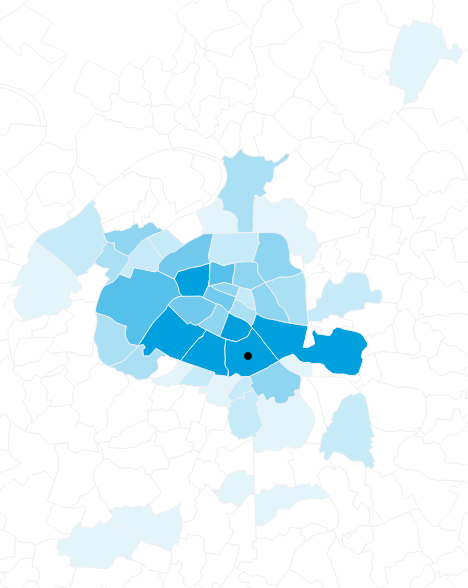
- Goal: Given the produced trips with their origin zone, define where they end = distribute the trips over a set of potential destination
Number of daily commutes arriving from 13th arrondissement
Four-step model: Trip distribution
- Based on trip generation, we want to predict the number of trips going from zone s to zone t
- Various ways to model flows between zones
- Gravity model
- Discrete choice model
-
Maximum entropy
- Can be formulated per group g.
F_{s,t} = f(X_s, X_t)
Flow between s and t
Model
| O1 | ... | ... | On | |
|---|---|---|---|---|
| D1 | ||||
| ... | Fst | |||
| ... | ||||
| Dn |
O_s
D_t
Four-step model: Trip distribution
- Growth factor approach
- Useful if information on existing flows is available for many relations and we want to obtain an explicative model
- Useful if information on existing flows is available for many relations and we want to obtain an explicative model
- Constrained approach
- We have little flow information, but know about the total in each zone (e.g. population and workplaces)
F_{s,t} = \lambda_{s,t} \cdot O_t
\lambda_{s,t} = f(X_s, X_t)
Trip generation
Growth factor modeled through zone attributes
D_t = \sum_s F_{s,t}
O_s = \sum_t F_{s,t}
F_{s,t} = f(X_s, X_t)
Require
with
Four-step model: Trip distribution
- Common approach: Gravity model
F_{s,t} = f(X_s, X_t) = \rho \cdot P_s \cdot A_t \cdot R_{s,t}
P_s = P(X_s)
A_t = A(X_t)
Production model, e.g. P = Population or Population Density
Attraction model, e.g. A = Workplaces or Workplace Density
R_{s,t} = A(X_s, X_t)
Resistance model, e.g. based on travel time or distance (also called impedance)
R_{s,t} = exp( -\beta \cdot \text{Distance}(s,t) )
Four-step model: Trip distribution
F_{s,t} = f(X_s, X_t) = \rho \cdot P_s \cdot A_t \cdot R_{s,t}
O_s = \sum_t F_{s,t}
O_s = \sum_t F_{s,t}
- Common approach: Gravity model
-
If we know F, we can calibrate all models, e.g. using OLS ...
- ... but we may better know required origins, i.e.
Four-step model: Trip distribution
F_{s,t} = f(X_s, X_t) = \rho \cdot P_s \cdot A_t \cdot R_{s,t}
O_s = \sum_t F_{s,t}
O_s = \sum_t F_{s,t} = \rho \cdot P_s \cdot \sum_t A_t \cdot R_{s,t}
- Common approach: Gravity model
-
If we know F, we can calibrate all models, e.g. using OLS ...
- ... but we may better know required origins, i.e.
Four-step model: Trip distribution
- Common approach: Gravity model
-
If we know F, we can calibrate all models, e.g. using OLS ...
-
... but we may better know required origins, i.e.
F_{s,t} = f(X_s, X_t) = \rho \cdot P_s \cdot A_t \cdot R_{s,t}
O_s = \sum_t F_{s,t}
O_s = \sum_t F_{s,t}
P_s = \frac{O_s}{\rho \sum_t A_t R_{s,t}}
Four-step model: Trip distribution
-
... which can be inserted into the model ...
-
... leading to
with
- If R is given or estimated independently (usually the case), the flows F are determined!
F_{s,t} = f(X_s, X_t) = \rho \cdot P_s \cdot A_t \cdot R_{s,t}
\alpha_s = \frac{1}{\sum_t A_t R_{s,t}}
F_{s,t} = f(X_s, X_t) = \alpha_s \cdot A_t \cdot R_{s,t} \cdot O_s
P_s = \frac{O_s}{\rho \sum_t A_t R_{s,t}}
Four-step model: Trip distribution
-
Including both origin and destination constraints gives
with
F_{s,t} = f(X_s, X_t) = \alpha_s \cdot \beta_t \cdot O_s \cdot D_t \cdot R_{s,t}
P_s = \frac{O_s}{\rho \sum_t A_t R_{s,t}}
\alpha_s = \frac{1}{\sum_t A_t R_{s,t}}
\beta_t = \frac{1}{\sum_s P_s R_{s,t}}
A_t = \frac{D_t}{\rho \sum_s P_s R_{s,t}}
- By construction, the origin and destination counts are replicated when iteratively solving
Four-step model: Mode choice
-
Goal: Given the infrastructure and the generated OD trips, which mode of transport should be used for them.
- Expressed as mode share: How many percent of the trips on a OD relation are performed with mode m?
P[m]
m \in \{ car, pt, ... \}
\sum_m P[m] = 1
P[m] \geq 0
Utility maximization
-
Utility maximization is important concept in transport planning: Given a set of choices (modes, destinations, ...) we can assign a utility v to each alternative k.
- We assume rational decision makers that always want to choose the alternative with the highest utility.
- Homo oeconomicus
v_k = \beta^T X
k^* = \text{arg max}_k \{ v_1, ..., v_k, ... v_K \}
Utility maximization
- Example: Choice between two public transport connections
v_k = \beta_\text{travelTime} \cdot x_{k, \text{travelTime}} + \beta_\text{interchanges} \cdot x_{k, \text{interchanges}}
Connection A
x_{A, \text{travelTime}} = 20\ \text{min}
Connection B
x_{B, \text{travelTime}} = 30\ \text{min}
x_{B, \text{interchanges}} = 0
x_{A, \text{interchanges}} = 1
-0.6
-1.0
-0.6 * 20 - 1.0 * 1 = -13
-0.6 * 30 - 1.0 * 0 = -19
Connection A is better alternative.
Utility maximization
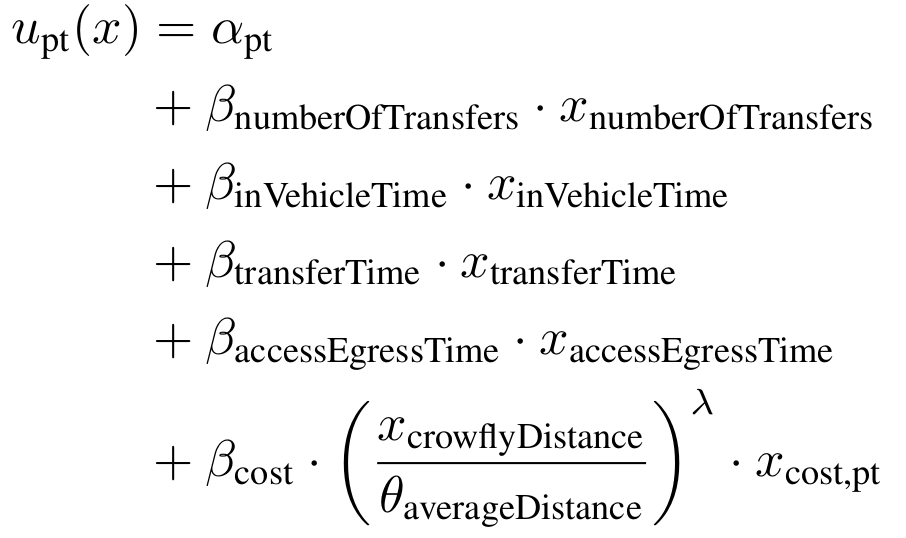
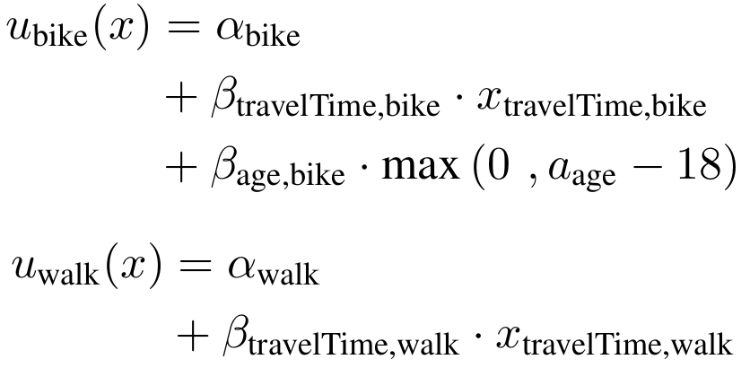
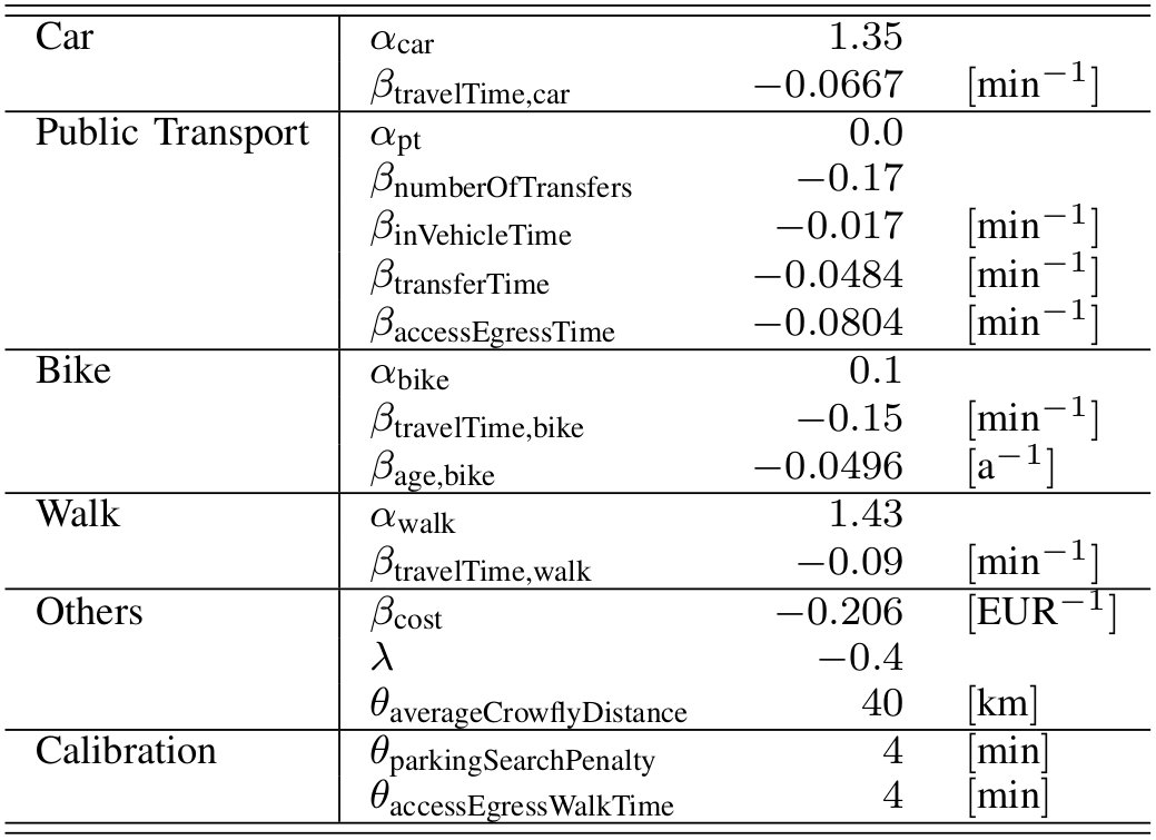
- Example: Mode choice model
Random Utility Models
- How to estimate such models?
- Assume K alternatives and N observed choices y described by index i.
- We want to find the set of parameters such that all choices i are replicated correctly:
v_k(X_i) = \beta^T \cdot X_k
y_i \in \{ 1, ..., K \}
\beta
y_i = \text{arg max}_k \{ v_k(X_i|\beta) \} \ \
\forall i
Find such that
Random Utility Models
- Not easily possible: We cannot model reality sufficiently well, people have own tastes.
- Hence, we introduce an error term.
- This leads to a random utility maximization (RUM) model
u_{k,i} = v_{k,i} + \sigma \epsilon_{k,i}
E[\epsilon_{k,i}] = 0
\sigma \geq 0
k^*_i = \text{arg max}_k \{ u_{k,i} \}
k^*_i = \{ k \ | \ (u_{k,i} \geq u_{1,i}) \land \ (u_{k,i} \geq u_{2,i}) \land ... \}
Random Utility Models
- McFadden has shown in the seventies that if error follows Extreme Value distribution ...
- ... there is a closed form expression for the choice probability:
- Two alternatives k:
Binomial logit model
- Multiple alternatives k:
Multinomial logit model
u_k = v_k + \sigma \epsilon_k
\epsilon_{k,i} \sim \text{IV}
P[k] = \frac{\exp(\sigma^{-1} v_k)}{\sum_{k'}\exp(\sigma^{-1} v_{k'})}
Random Utility Models
- Coming back to estimation:
- Under multinomial logit assumption, we can write a (log-)likelihood function ...
- ... which is proven convex and can be maximized using any optimization method!
P[k] = \frac{\exp(\sigma^{-1} v_k)}{\sum_{k'}\exp(\sigma^{-1} v_{k'})}
v_k(X_i) = \beta^T \cdot X_k
y_i \in \{ 1, ..., K \}
\mathcal{L}(\beta) = \prod_i P[y_i|X_i,\beta]
l(\beta) = \sum_i \log P[y_i|X_i,\beta]
\beta^* = \text{arg max}_{\beta} \sum_i \log P[y_i|X_i,\beta]
Random Utility Models
- Multinomial logit is commonly used and part of larger class of discrete choice models.
- Can also be used in distribution step.
- Last step of 4S model
- What are resulting flows on the roads?
- What are the resulting travel times?
Four-step model: Assignment
- Again, based on rational decision maker
- Game theoretic perspective: Travellers compete about using the roads, each maximizing the utility they gain
- Many ways of solving assignment problem
Four-step model: Assignment
- Example: Two routes
- Travellers on Route A:
- Travellers on Route B:
- Total travellers from S to E:
- Travel time route A (normal road):
- Travel time route B (highway):
- Wardrop principle: Travellers tend to minimize their travel time.
Four-step model: Assignment
S
E
Route A
Route B
n_{A}
n_{B}
N = n_{A} + n_{B}
t_A(n_A) = 500 + n_A \cdot 2
t_B(n_B) = 1000 + n_B \cdot 1
How many people use each road? What are the travel times?
- Example: Two routes
- If travel time on A is shorter than B, people would switch to B, and vice versa. Hence, travel times, must be in equilibirum!
- This gives
- If travel time on A is shorter than B, people would switch to B, and vice versa. Hence, travel times, must be in equilibirum!
Four-step model: Assignment
S
E
Route A
Route B
n_{B}
N = n_{A} + n_{B}
t_A(n_A) = 500 + n_A \cdot 2
t_B(n_B) = 1000 + n_B \cdot 1
n_{A}
t_A(n_A) = t_B(n_B)
500 + 2 \cdot n_A = 1000 + 1 \cdot n_B
n_A = N - n_B
(*)
from (**)
(**)
N = 1000
n_A = 433.33
n_B = 566.66
t_A = t_B = 1366.66
- What about many different routes between two points?
- What about many different start/end points in a network?
- Wardrop defined general formulation, leading to a game-theoretic Nash equilibrium
Four-step model: Assignment
\text{min}_x \sum_a \int_0^{x_a} t_a(x_a) \text{d}x
\sum_k f_k^{rs} = q_{rs} \ \ \ \forall r, s
x_a = \sum_r \sum_s \sum_k \delta^{rs}_{k,a} f_k^{rs} \ \ \ \forall a
f_k^{rs} \geq 0
x_a \geq 0
s.t.
Four-step model: Assignment
- So far, Static Traffic Assignment (STA): Departure time of vehicles does not matter (we look at peak our time slice).
- Methods for Dynamic Traffic Assignment (DTA) exist, which consider detailed movements of vehicles, traffic lights, ...
Four-step model: Feedback
Generation
Distribution
Mode choice
Assignment
- Now travel times in the network are known. They can be fed back to the distribution stage (which travel times did we assume back then)?
- 4S model can be run iteratively to bring stages in equilibrium.
- Many caveats in terms of consistency and convergence (beyond the scope in this lecture).
Activity-based models
- Non-equilibrium models
- Sequential decisions during simulation for each agent
- Dynamic reaction to environment
Activity-based models
Activity 1
Activity 2
Activity 3
Decision
Decision
Analysis
Person 1
Activity 1
Activity 2
Person 1
Decision
- Non-equilibrium models
- Sequential decisions during simulation for each agent
- Dynamic reaction to environment
- Equilibrium models
- Decision made for a whole day
- All decisions of persons go into equilibrium after multiple iterations
Activity-based models
Activity 1
Activity 2
Activity 3
Person 1
Activity 1
Activity 2
Person 1
Analysis
Decision making
Iterations
- Non-equilibrium models
- Sequential decisions during simulation for each agent
- Dynamic reaction to environment
- Equilibrium models
- Decision made for a whole day
- All decisions of persons go into equilibrium after multiple iterations
- Hybrid models
Activity-based models
- Generally, detailed input data is needed to reach at detailed output
- Data processing similar to 4S models, but much more complex and some components are dynamically treated in the simulation
Activity-based models
-
Population synthesis
The task is to create a synthetic representation of the population with socio-demographical households and person attributes
- Multitude of approaches
- Iterative Proportional Fitting (IPF)
- Iterative Proportional Updating (IPU)
- Gibbs Sampling
Activity-based models
-
Population synthesis
The task is to create a synthetic representation of the population with socio-demographical households and person attributes
- Multitude of approaches
- Iterative Proportional Fitting (IPF)
- Iterative Proportional Updating (IPU)
- Gibbs Sampling
- Bayesian Networks
Activity-based models
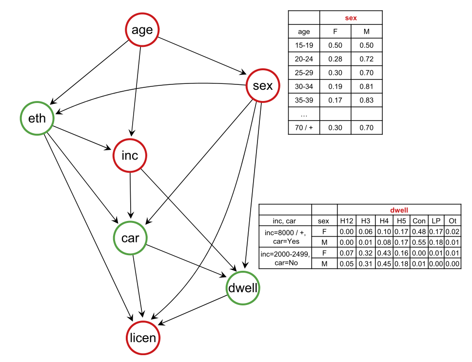
Sun, L., Erath, A., 2015. A Bayesian network approach for population synthesis. Transportation Research Part C: Emerging Technologies 61, 49–62. https://doi.org/10.1016/j.trc.2015.10.010
-
Population synthesis
The task is to create a synthetic representation of the population with socio-demographical households and person attributes
- Multitude of approaches
- Iterative Proportional Fitting (IPF)
- Iterative Proportional Updating (IPU)
- Gibbs Sampling
- Bayesian Networks
- Hidden Markov Models
Activity-based models
Saadi, I., Mustafa, A., Teller, J., Farooq, B., Cools, M., 2016. Hidden Markov Model-based population synthesis. Transportation Research Part B: Methodological 90, 1–21. https://doi.org/10.1016/j.trb.2016.04.007
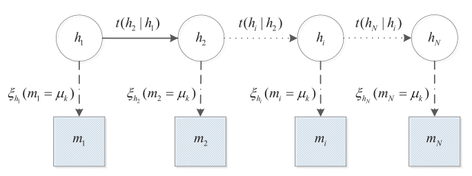
-
Population synthesis
The task is to create a synthetic representation of the population with socio-demographical households and person attributes
- Multitude of approaches
- Iterative Proportional Fitting (IPF)
- Iterative Proportional Updating (IPU)
- Gibbs Sampling
- Bayesian Networks
- Hidden Markov Models
- Deep Generative Modeling
Variational Auto Encoders
Activity-based models
Borysov, S.S., Rich, J., Pereira, F.C., 2019. How to generate micro-agents? A deep generative modeling approach to population synthesis. Transportation Research Part C: Emerging Technologies 106, 73–97. https://doi.org/10.1016/j.trc.2019.07.006
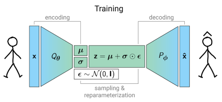
-
Synthesis of activity chains
Given sociodemographic attributes, generate daily activity chains for the agents.
- Today increasingly use of GPS / GSM trace data sets to train models
- Some examples
- Statistical Matching Approaches
- Skeleton-based approaches
- Sequential choice models (classic approach)
- Sequential Alignment Methods (SAM)
- Bayesian Networks
- ...
Activity-based models
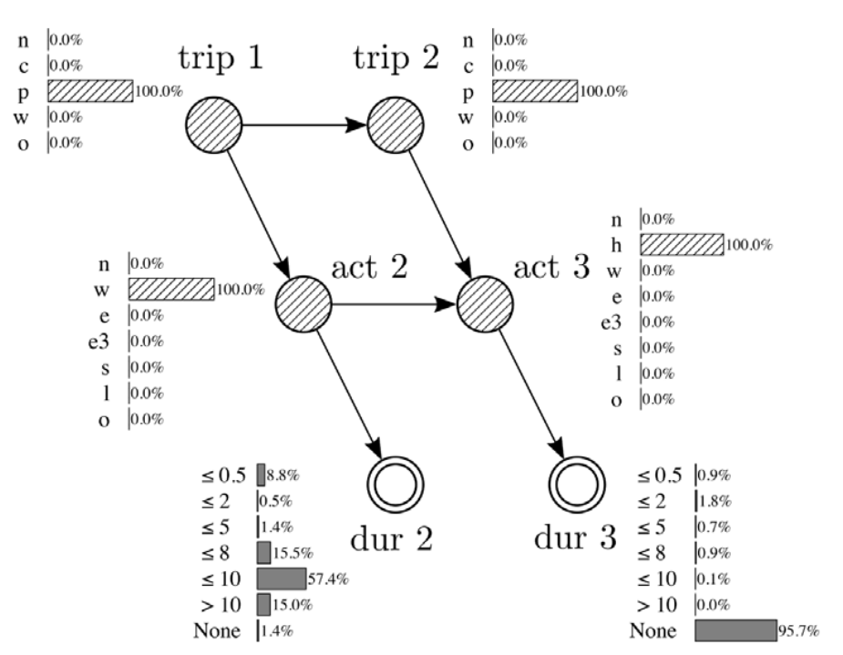
Joubert, J.W., de Waal, A., 2020. Activity-based travel demand generation using Bayesian networks. Transportation Research Part C: Emerging Technologies 120, 102804. https://doi.org/10.1016/j.trc.2020.102804
-
Further aspects:
- Departure times from activities
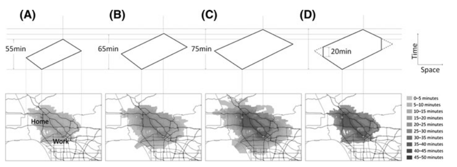
- Locations of activities
- Potential Path Areas (PPA)
- Space-time prisms
- ...
Activity-based models
Yoon, S.Y., Deutsch, K., Chen, Y., Goulias, K.G., 2012. Feasibility of using time–space prism to represent available opportunities and choice sets for destination choice models in the context of dynamic urban environments. Transportation 39, 807–823. https://doi.org/10.1007/s11116-012-9407-8
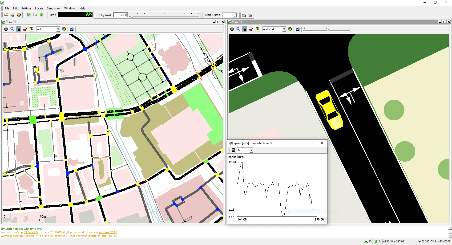
- As is demand generation, mobility simulation is often also more complex
- Usually agent-based
- Microscopic simulation
- VISSIM, SUMO, ...
- VISSIM, SUMO, ...
- Mesoscopic simulation
- MATSim, SimMobility,
POLARIS, ...
- MATSim, SimMobility,
Activity-based models
- Convergence
- Usually based on utility maximization principle
- Detection of Nash equilibria
- Output metric convergence
- Calibration
- Complex simulator (no closed form expression)
- Noisy output (needs stochastic optimization)
- Large run-times
Activity-based models: Challenges
- Last semester
- Example with eqasim (for demand synthesis)
- and MATSim (traffic simulation)
Activity-based models: Example
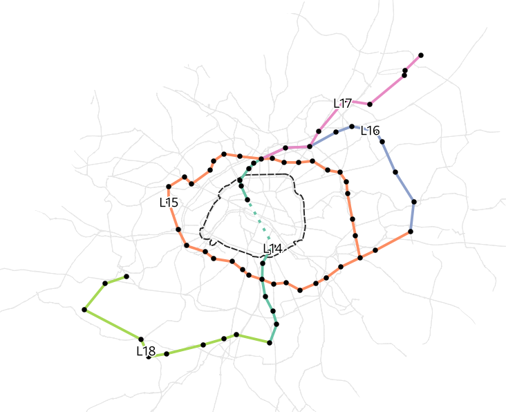
Grand Paris Express
- One of largest infrastructure projects in Europe
- Affecting mobility behaviour of large share of population in Île-de-France
Course project
- Learn more about Grand Paris Express
- Simple demand estimate for Grand Paris Express and its impact on existing public transport
- Four groups:
- Demand
- Routing
- GTFS
- Mode choice
Course project
Demand
GTFS
Routing
Mode choice
- Estimate commuting
demand based on census - Look into weighting and down-scaling
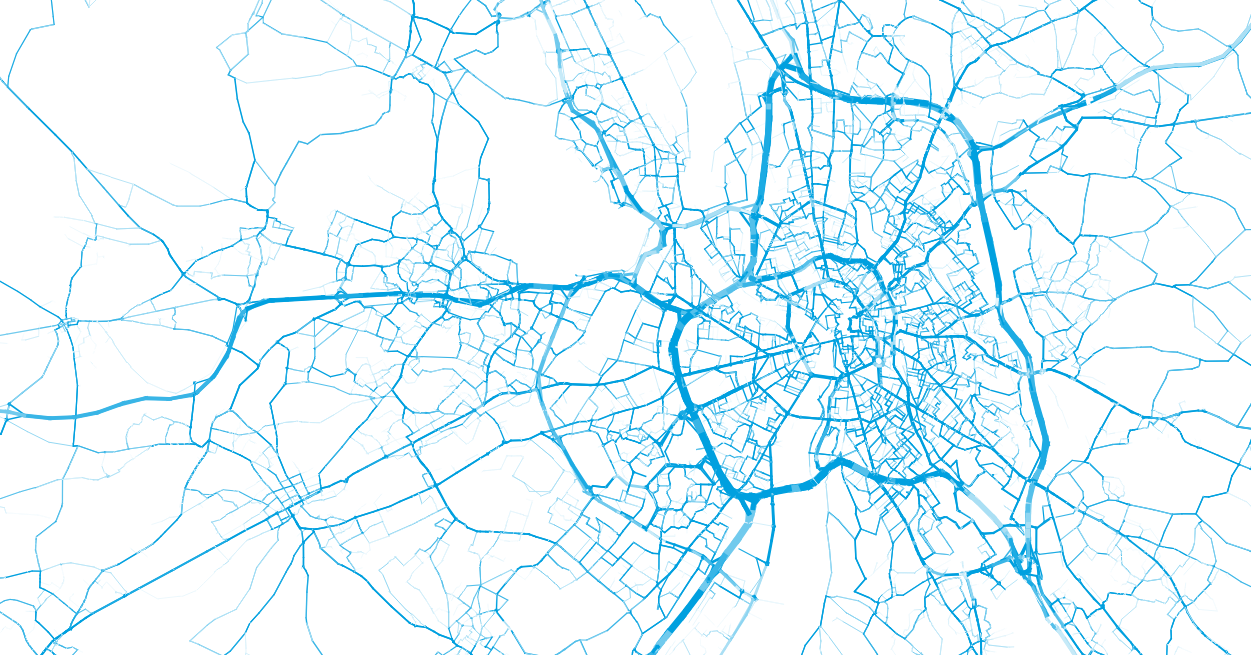
- Visualize commuting
demand
- Understand GTFS format
- Integrate Grand Paris Express in digital transit schedule
- Visualize network
- Use routing software to calculate commuting trip characteristics today and with Grand Paris Express
- Understand delays in car traffic
- Visualize high-level routing metrics
- Use multinomial logit model to analyze mode choice for commuting trips
- Visualize difference from reference data and mode use on a map
- Coordination within each group
- Coordination across groups
Course project
Demand
GTFS
Routing
Mode choice
- Estimate commuting
demand based on census - Look into weighting and down-scaling
- Visualize commuting
demand
- Understand GTFS format
- Integrate Grand Paris Express in digital transit schedule
- Visualize network
- Use routing software to calculate commuting trip characteristics today and with Grand Paris Express
- Understand delays in car traffic
- Visualize high-level routing metrics
- Use multinomial logit model to analyze mode choice for commuting trips
- Visualize difference from reference data and mode use on a map
- Demand analysis: Where does GPE have the highest impact (in travel time improvements and in actual mode-choice-based use)?
- Supply analysis: Which existing lines loose how many users? How many users do the new lines have compared to existing lines?
Course project (Information flow)
Demand
GTFS
Routing
Mode choice
- Identifier
- Origin/destination locations
- Total flow between OD
- Reference mode shares
For instance, count how many commutes make use of RER A before and after including the Grand Paris Express.
- GTFS scheduled enriched with Grand Paris Express
- Identifier
- Car/Public transport travel time
- Public transport line switches
- Public transit lines
- Identifier
- Chosen mode
Group: Demand
-
Technical task: Produce a commuting data set for Île-de-France as a list of trips with origin coordinate, destination coordinate, current mode shares, and the total number of commuters.
-
Analysis task:
- Visualize the number of trips in each municipality on a map
- Visualize the number of people using car vs. public transport in those municipalities. Which patterns do you observe in Île-de-France?
Group: Demand
-
Recommendations
- Investigate the French census commuting data set
https://www.insee.fr/fr/statistiques/3566008
- Read the documentation of the data. It will give you the flows from one municipality to another.
- Be careful with Paris, which is encoded as one municipality, but information on the arrondissement is available!
- Take into account the weight column (PONDI), because every row represent X trips in reality.
- Consider the modes "car" and "public transport" and denote the rest as "other".
- Investigate the French census commuting data set
Group: Demand
-
Recommendations
- Spatial information can be obtained from IGN:
https://geoservices.ign.fr/contoursiris
- The data represents IRIS (finer zoning system than municipalities), you need to join them to municipalities.
- Use the centroids of the municipalities as representative origin-destination points for the trip to route.
- Take care of the coordinate reference system (CRS), which is the French standard one (EPSG:2154), but routing needs coordinates in longitude / latitude (EPSG:4326)
- Spatial information can be obtained from IGN:
Group: Routing
-
Technical task: Set up a system that allows you to route trips in Île-de-France with a start coordinate, and an end coordinate such that you obtain the travel time by car, travel time by public transport and potentially other attributes that are of interest. Take into account that during the morning peak hour, roads are congested!
-
Analysis task:
- Given a set of trips (provided by "demand" group), show the distribution of travel times by car and public transport in Île-de-France. Where are regions where travelling by car is generally quicker or slower?
Group: Routing
-
Recommendations
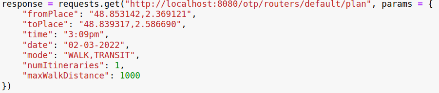
- Usually, we would use API services like HERE, Bing or Google. There, we can send (start, end) coordinates and receive travel times, number of transfers, etc. for all modes of transport
- Here, we also want to look into the future transport system.
- You can use OpenTripPlanner, but also any other routing software if you prefer. OpenTripPlanner provides an easy REST interface.
- Usually, we would use API services like HERE, Bing or Google. There, we can send (start, end) coordinates and receive travel times, number of transfers, etc. for all modes of transport
Group: Routing
-
Recommendations
- For the road network, you need OpenStreetMap data for Île-de-France:
https://download.geofabrik.de/europe/france/ile-de-france.html
- The baseline (current) transit schedule is provided by IDFM:
https://data.iledefrance-mobilites.fr/explore/dataset/offre-horaires-tc-gtfs-idfm/information/
- For the road network, you need OpenStreetMap data for Île-de-France:
Group: Routing
-
Recommendations
- Note that OpenTripPlanner has no information about congestion in the morning. How can you solve this problem?
- Easy solution: Check a couple of trips in Île-de-France by using the free flow travel time provided by OpenTripPlanner and compare them to the calculated travel time by Bing or Google Maps at 08h00. Note down an average scaling factor an apply it to your calculated travel time.
- Note that OpenTripPlanner has no information about congestion in the morning. How can you solve this problem?
Group: GTFS
-
Technical task: Get familiar with the structure of a digital transit schedule in GTFS format. The group "Routing" will be able to use this data to find routes of passengers with this data. Integrate the new Metro lines of the Grand Paris Express into the GTFS file of Île-de-France.
-
Analysis task:
- Visualize the Metro network (lines and stations) of Paris before and after including the Grand Paris Express on a map.
Group: GTFS
-
Recommendations
- You can find a valid baseline (current) GTFS schedule from IDFM
https://data.iledefrance-mobilites.fr/explore/dataset/offre-horaires-tc-gtfs-idfm/information/
- Detailed information on GTFS is available from the GTFS specification
https://developers.google.com/transit/gtfs/
- Open data from the Grand Paris Express is available here
https://www.data.gouv.fr/fr/organizations/societe-du-grand-paris/#datasets
- You can find a valid baseline (current) GTFS schedule from IDFM
Group: GTFS
-
Recommendations
- Attention! Is there any data missing? Are there any errors in the provided data sets? Inconsistencies? Do not stick too long to those problems, but try to find an easy and pragmatic solution. It is fine to report your findings in the presentations, no need to fix everything in detail!
- How are transfers between lines represented in GTFS? Do they need special treatment when implementing the Grand Paris Express?
- Attention! Is there any data missing? Are there any errors in the provided data sets? Inconsistencies? Do not stick too long to those problems, but try to find an easy and pragmatic solution. It is fine to report your findings in the presentations, no need to fix everything in detail!
Group: Mode choice
-
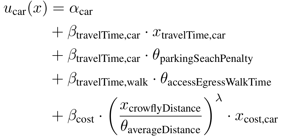
Technical task: Set up a discrete mode choice model on commuting data for Île-de-France. Propose a model that makes it possible to perform a prediction based on car travel time and public transport connection characteristics.
-
Analysis task:
- Visualize the use of car and public transport as the commuting mode in Île-de-France on a map or as aggregate statistics.
- Visualize the differences you see with different modelling assumptions.
Group: Mode choice
-
Recommendations
- You can find information on existing mode choice models for Île-de-France: https://www.sciencedirect.com/science/article/pii/S2352146515001180
- The groups "Demand" and "Routing" will provide you with a ground truth that you can use to estimate a predictive model. The model should predict the mode share for a origin-destination relation that is characterized by trip attributes:
- You can find information on existing mode choice models for Île-de-France: https://www.sciencedirect.com/science/article/pii/S2352146515001180
Car Mode Share
PT Mode Share
Other Mode Share
Car travel time
PT travel time
Car distance / cost
PT distance / cost
PT transfers
... ? ...
Group: Mode choice
-
Recommendations
- The easy approach is to use a Multinomial Logit Model and fit it using a least-squares optimization (you may need to weight by the total demand per OD relation). But you may also test alternative models, e.g. machine learning models, neural networks, ...
- The "Mode choice" group is rather dependent on the inputs from the other groups. To start quickly, collect a couple of trips with random origin and destination locations through Google Maps or Bing (up to 100) and try to develop the model infrastructure with them.
- The easy approach is to use a Multinomial Logit Model and fit it using a least-squares optimization (you may need to weight by the total demand per OD relation). But you may also test alternative models, e.g. machine learning models, neural networks, ...
Final analysis
- Group "Routing" performs a routing of the trips provided by Group "Demand" given the original Île-de-France transit schedule, and then with the updated transit schedule provided by group "GTFS". After, group "Mode choice" performs a mode choice experiment for the provided trips, obtaining the mode share before and after including the Grand Paris Express.
-
Analysis task:
- Which OD relations decrease most in travel time when the Grand Paris Express is implemented without considering mode shares? How to visualize this?
- Which areas in Île-de-France show the strongest changes in mode usage?
- Assess and visualize the daily number of users of the new and existing Metro lines, RER lines and Transilien in a before-after comparison.
-
Final presentation including all groups. During the presentation, each group presents their results. At the end, the final demand analysis combining all partial results is presented. The presentation date is 25 March.
- Grading:
- Results: It is not expected to achieve perfect results. Focus should be put on which components worked well, and where you have encountered difficulties. Grading is based on the quality of presenting those reflections.
- Visual consistency: Make sure to coordinate on the visual appearance of the whole presentation. Grading will be based on how well the groups manage to stick to an overall scheme.
- Each group receives one grade for their presentation.
- Results: It is not expected to achieve perfect results. Focus should be put on which components worked well, and where you have encountered difficulties. Grading is based on the quality of presenting those reflections.
Deliverables & Grading
-
Group report of 2-3 pages. To be submitted until 22 April.
- Grading:
- Focus is on reflection.
- (1) On teamwork: Write about how you were working together within your group and across the groups. Reflect on what went well, what went not ideally. What did you learn in terms of working together in a project?
- (2) On your group task: Which elements were difficult? Where can the analysis be improved and how? What data did you exchange with other groups, how did you define the formats? Describe the methodology you have used. What approaches did you assess? Why did you choose a specific one? What were your selection criteria?
- (1) On teamwork: Write about how you were working together within your group and across the groups. Reflect on what went well, what went not ideally. What did you learn in terms of working together in a project?
- Focus is on reflection.
Deliverables & Grading
Timeline
-
Today: Defining groups
-
18 February:
- Intermediate presentation of initial analyses (no need to prepare slides)
- Q&A, exchange among the groups
-
11 March:
- Presentation of developments in each group (no slides needed)
- Coordination across groups for final project
-
25 March
- Final presentation
Please register for the groups:

Course: Grand Paris Express Project
By Sebastian Hörl


