1.7 Sigmoid Neuron
The building block of Deep Neural Networks
Recap: Six jars
What we saw in the previous chapter?
(c) One Fourth Labs
Repeat the slide where we summarise the perceptron model in the context of the 6 jars.
Some thoughts on the contest
Just some ramblings!
(c) One Fourth Labs
We should create the binary classification monthly contest such that we can somehow visualize that the data is not linearly separable (don't know how)
We should also be able to visualize why the perceptron model is not fitting
Also give them some insights into what does the loss function indicate and how to make sense of it
Limitations of Perceptron
Can we plot the perceptron function ?
(c) One Fourth Labs
1. Show a training matrix with only 1 input (salary) and the decision is buy_car/not_buy_car
4. First only show x and y axis, label x axis as salary and y-axis as "\hat{y} = \hat{f}(salary)= perceptron(salary)"
5. Now take a positive point from the training data. Mark it on the x-axis and then mark the corresponding output for this point (+1)
6. Do this for a few points and then draw the step function
7, 8. Show the cartoon
9. Now on the x-axis show red and green regions for the positive and negative points
2. Show the perceptron model equations here
3. Suppose w=2, b =1 (comments for Mitesh: I took linearly separable data

7. Wait a minute!
8. Doesn't the perceptron divide the input space into positive and negative halves

Limitations of Perceptron
Can we plot the perceptron function ?
(c) One Fourth Labs
Wait a minute!
| Salary ( in thousands) | Can buy a car? |
|---|---|
| 80 | 1 |
| 20 | 0 |
| 65 | 1 |
| 15 | 0 |
| 30 | 0 |
| 49 | 0 |
| 51 | 1 |
| 87 | 1 |
Doesn't the perceptron divide the input space into positive and negative halves ?
y=\sum_{i=1}^n w_i x_i \geq b
\text{Suppose,} \\
\mathbb{w_1} = 2,\\
\hspace{-0.2cm}\mathbb{b}\ \ = 1


Limitations of Perceptron
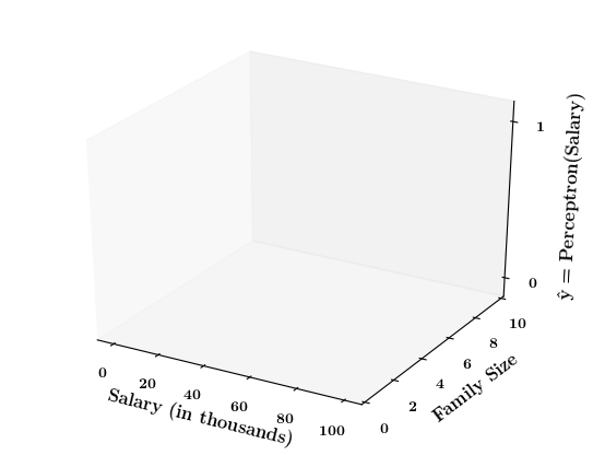
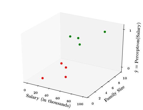
How does the perceptron function look in 2 dimensions?
(c) One Fourth Labs
1. Show a training matrix with only 2 inputs (salary, family size) and the decision is buy_car/not_buy_car
4. First only show x1, x2 and y axis, label x1 axis as salary, x2 axis as family size and y-axis as "\hat{y} = \hat{f}(salary, size)= perceptron(salary, size)"
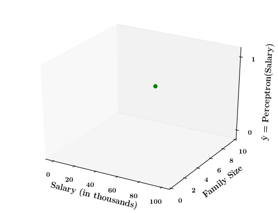
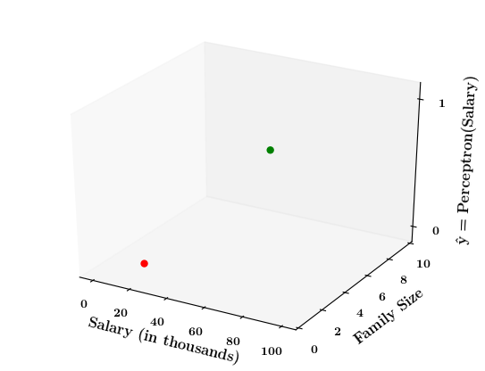
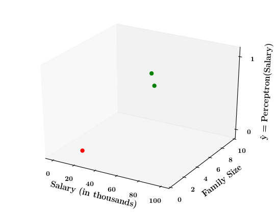
5. Now take a positive point from the training data. Mark it on the x1,x2-plane and then mark the corresponding output for this point (+1)
6. Do this for a few points and then draw the 2d - step function
7. Now on the x1, x2 plane show red and green regions for the positive and negative points an show that the line which is the foot of the step function which divides the space into two halves
2. Show the perceptron model equations here
3. Suppose w_1=<some_value>, w_2=<some_value>, b =1
Limitations of Perceptron
How does the perceptron function look in 2 dimensions?
(c) One Fourth Labs
y=\sum_{i=1}^n w_i x_i \geq b
\text{Suppose,} \\
\mathbb{w_1} = 0.2,\\
\hspace{-0.2cm}\mathbb{w_2} = 0.1 \\
\mathbb{b} = -10.5
| Salary (in thousands) | Family size | Can buy a car? |
|---|---|---|
| 80 | 2 | 1 |
| 20 | 1 | 0 |
| 65 | 4 | 1 |
| 15 | 7 | 0 |
| 30 | 6 | 0 |
| 49 | 3 | 0 |
| 51 | 4 | 1 |
| 87 | 8 | 1 |
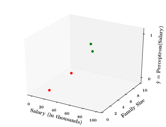
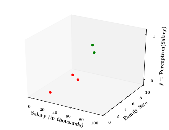
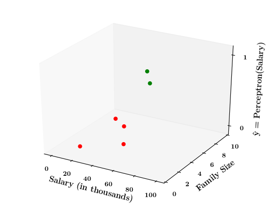
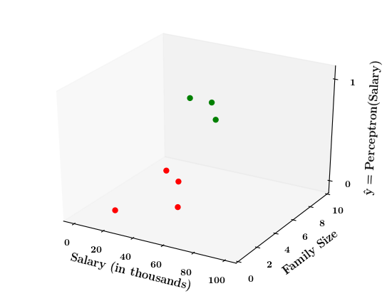

Limitations of Perceptron
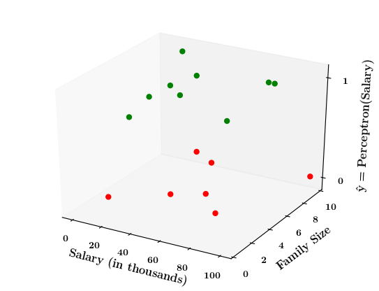
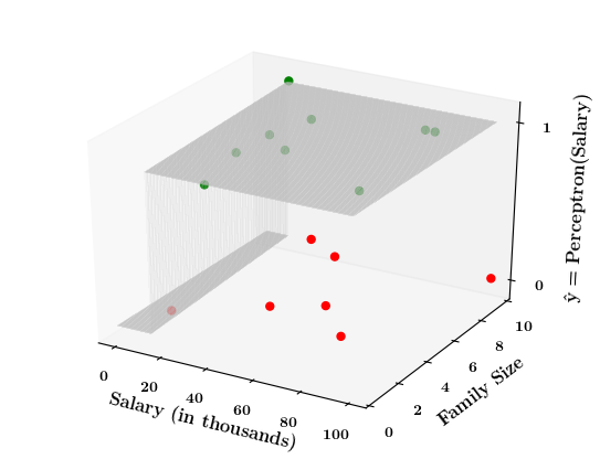
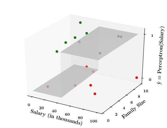
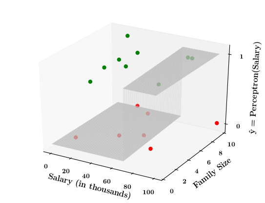
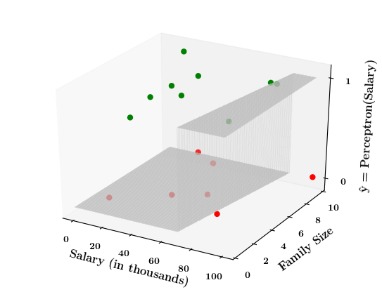
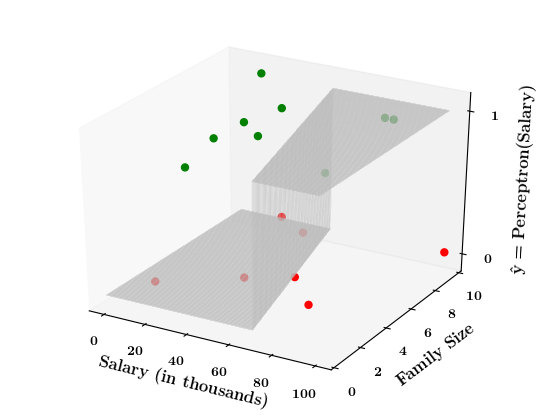
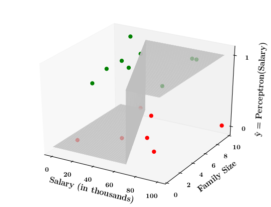
What if the data is not linearly separable ?
(c) One Fourth Labs
1. Show a training matrix with only 2 inputs (salary, family size) and the decision is buy_car/not_buy_car
Now on the x1. x2 plane show some data which is not linearly separable
Adjust the perceptron function and show that no matter what you do some green points will go to the other side or some red points will go to the other side.
2. Show the perceptron model equations here
3. Suppose w_1=<some_value>, w_2=<some_value>, b =1
Limitations of Perceptron
What if the data is not linearly separable ?
(c) One Fourth Labs
y=\sum_{i=1}^n w_i x_i \geq b
\text{Suppose,} \\
\mathbb{w_1} = 0.2,\\
\hspace{-0.2cm}\mathbb{w_2} = 0.1 \\
\mathbb{b} = -6
| Salary (in thousands) | Family size | Can buy a car? |
|---|---|---|
| 81 | 8 | 1 |
| 37 | 9 | 0 |
| 34 | 5 | 1 |
| ... | ... | ... |
| 40 | 4 | 0 |
| 100 | 10 | 0 |
| 10 | 10 | 1 |
| 85 | 8 | 1 |
\text{Suppose,} \\
\mathbb{w_1} = 0.2,\\
\hspace{-0.2cm}\mathbb{w_2} = 0.1 \\
\mathbb{b} = -3
\text{Suppose,} \\
\mathbb{w_1} = 0.2,\\
\hspace{-0.2cm}\mathbb{w_2} = -0.3 \\
\mathbb{b} = -14
\text{Suppose,} \\
\mathbb{w_1} = 0.2,\\
\hspace{-0.2cm}\mathbb{w_2} = -0.5 \\
\mathbb{b} = -14
\text{Suppose,} \\
\mathbb{w_1} = 0.2,\\
\hspace{-0.2cm}\mathbb{w_2} = 0.1 \\
\mathbb{b} = -9
\text{Suppose,} \\
\mathbb{w_1} = 0.2,\\
\hspace{-0.2cm}\mathbb{w_2} = 0.1 \\
\mathbb{b} = -14
\text{Suppose,} \\
\mathbb{w_1} = 0.2,\\
\hspace{-0.2cm}\mathbb{w_2} = -0.7 \\
\mathbb{b} = -14
\text{Suppose,} \\
\mathbb{w_1} = 0.2,\\
\hspace{-0.2cm}\mathbb{w_2} = 0.3 \\
\mathbb{b} = -14
\text{Suppose,} \\
\mathbb{w_1} = 0.2,\\
\hspace{-0.2cm}\mathbb{w_2} = 0.7 \\
\mathbb{b} = -14


Limitations of Perceptron
Isn't the perceptron model a bit harsh at the boundaries ?
(c) One Fourth Labs
Repeat the training data with one input (salary)
Show the 2d plot from before
2. Now show the cartoon
Show the perceptron model equations here
Suppose w_1=<some_value>, w_2=<some_value>, b =1
Isn't it a bit odd that a person with 150K salary will but a car but someone with 150.1K will not buy a car ?
Limitations of Perceptron
Isn't the perceptron model a bit harsh at the boundaries ?
(c) One Fourth Labs
Isn't it a bit odd that a person with 50.1K salary will buy a car but someone with 49.9K will not buy a car ?
| Salary ( in thousands) | Can buy a car? |
|---|---|
| 80 | 1 |
| 20 | 0 |
| 65 | 1 |
| 15 | 0 |
| 30 | 0 |
| 49 | 0 |
| 51 | 1 |
| 87 | 1 |
y=\sum_{i=1}^n w_i x_i \geq b
\text{Suppose,} \\
\mathbb{w_1} = 2,\\
\hspace{-0.2cm}\mathbb{b}\ \ = 1
The Road Ahead
What's going to change now ?
(c) One Fourth Labs
Show the six jars and convey the following by animation
-- Boolean output gets replaced by real output
-- "specific learning algo" gets replaced by "a more generic learning algorithm"
-- "harsh at boundaries gets replaced by smooth at boundaries
-- "Linear" gets replaced by non-linear
Harsh at boundaries
Linear
Real inputs
Boolean output
Specific learning algorithm
(c) One Fourth Labs
The Road Ahead
What's going to change now ?
(c) One Fourth Labs
\( \{0, 1\} \)
Boolean


Accuracy=\frac{\text{Number of correct predictions}}{\text{Total number of predictions}}
Loss
Model
Data
Task
Evaluation
Learning
Linear
Real inputs
Boolean output
loss = \sum_i max(0,1-y_i*\hat{y_i})
Specific learning algorithm
Harsh at boundaries
Real output
Non-linear
A more generic learning algorithm
Smooth at boundaries
Data and Task
What kind of data and tasks can Perceptron process ?
(c) One Fourth Labs
Same mobile phone dataset from before.
Real inputs
Data and Task
What kind of data and tasks can Perceptron process ?
(c) One Fourth Labs
Data and Task
What kind of data and tasks can Perceptron process ?
(c) One Fourth Labs
Real inputs
| Launch (within 6 months) | 0 | 1 | 1 | 0 | 0 | 1 | 0 | 1 | 1 |
| Weight (g) | 151 | 180 | 160 | 205 | 162 | 182 | 138 | 185 | 170 |
| Screen size (inches) | 5.8 | 6.18 | 5.84 | 6.2 | 5.9 | 6.26 | 4.7 | 6.41 | 5.5 |
| dual sim | 1 | 1 | 0 | 0 | 0 | 1 | 0 | 1 | 0 |
| Internal memory (>= 64 GB, 4GB RAM) | 1 | 1 | 1 | 1 | 1 | 1 | 1 | 1 | 1 |
| NFC | 0 | 1 | 1 | 0 | 1 | 0 | 1 | 1 | 1 |
| Radio | 1 | 0 | 0 | 1 | 1 | 1 | 0 | 0 | 0 |
| Battery(mAh) | 3060 | 3500 | 3060 | 5000 | 3000 | 4000 | 1960 | 3700 | 3260 |
| Price (INR) | 15k | 32k | 25k | 18k | 14k | 12k | 35k | 42k | 44k |
| Like (y) | 1 | 0 | 1 | 0 | 1 | 1 | 0 | 1 | 0 |


Model
Can we have a smoother (not-so-harsh) function ?
(c) One Fourth Labs
1) Show step function first and then super-impose the sigmoid function
2) Show the equation
3) Now on the RHS below the equation, substitute some values for wx+b and show the output on the plot (basically, I want to tell people that don't get overwhelmed when you see a function, just susbstitute some values in it and see how the plot looks, 0,1,-1, \inf, -inf
Show the sigmoid function equation here
Model
What happens when we have more than 1 input ?
(c) One Fourth Labs
1) Show the same phone data from before
2) Now show an image of sigmoid model with the equation containing \sum_w_i x_i + b
3) Now replace the summation by w^Tx
4) How do you plot this function: on x-axis show w^tx +b and on y-axis show the output y (again plot for different values of w^tx +b)
Show the sigmoid function equation here
Model
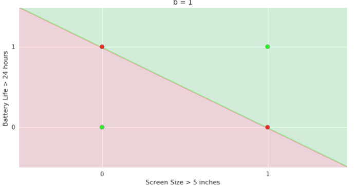
How does this help when the data is not linearly separable ?
(c) One Fourth Labs
Still does not completely solve our problem but we will slowly get there!
1. Show a training matrix with only 2 inputs (salary, family size) and the decision is buy_car/not_buy_car
1. In the first case we will consider data which only ha problems at the boundary (meaning that only at the boundary around wx+b = 0 some green and red points mix with each other)
2. Now show that unlike the perceptron which was either misclassifying the positive or negative points, sigmoid gives a soft decision
3. also show that by adjusting w_1 and w_2 you can accommodate for different types of boundary cases (please take Gokul's help for these plots)
2. Show the sigmoid model equations here
Model
What about extreme non-linearity ?
(c) One Fourth Labs
Still does not completely solve our problem but we will slowly get there with more complex models!
1. Show a training matrix with only 2 inputs (salary, family size) and the decision is buy_car/not_buy_car
1.Now show a case where the blue and red points are completely mixed with each other
2. show that no matter how you adjust w_1 and w_2 you will not be able to find any separation between blue and red points
3. Now show the quote at RHS bottom using our cartoon person
2. Show the sigmoid model equations here
Model
How does the function behave when we change w and b
(c) One Fourth Labs
5. Cartoon person: At what value of x is the value of sigmoid(X) = 0.5
2. Show a scale here for w and b
1. Show the sigmoid function here (the x-axis is x and y -asix is sigmoid(x)
3. CHange the value of w below and show how the plot changes
4. Now change the value of w below and show how the plot changes
5. Show the cartoon person woth the W
6. the derivation
2. Show the sigmoid model equations here
the derivation to show that sigm(x) = 0.5 at x = -b/w
Loss Function
What is the loss function that you use for this model ?
(c) One Fourth Labs
1. Show small training matrix here
2. On RHS show the model equation an y_hat = sigmoid
3. Show an empty column for y_hat now and then add entries in it (numbers between 0 and 1)
4. Now on RHS below the model equations show the equation for sqaured error loss
5. Now using the cartoon person show that we can use even better loss functions in this case but we will see that later in the course.
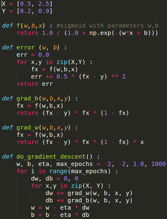
Learning Algorithm
Can we take a closer look at what we just did ?
(c) One Fourth Labs
Initialise
1. Start with the same algo as on previous slide
2. Replace guess_and_update by w = w+\delat w and b = b + \delata b
3. In this box now show the plot again containing all the points and show how you were going over them one by one in the algo on LHS
4. now below this box, write \delta w= some_guess, \deltab = some_guess
\(w_1, w_2, b \)
Iterate over data:
\( \mathscr{L} = compute\_loss(x_i) \)
\( update(w_1, w_2, b, \mathscr{L}) \)
till satisfied
Learning Algorithm
Can we connect this to the loss function ?
(c) One Fourth Labs
Initialise
0. Same algo as on previous slide
1. Show a table containing iteration number, w, b, loss
2. In this black box show the plot again
3. Now sync the table and the plot such that you show the w,b value in the table at the end of each iteration and show how the corresponding loss looks like and how the plot looks like
4. In apink box below say "Indeed we were using the loss function to guide us in finding \delta w and \delta b
\(w_1, w_2, b \)
Iterate over data:
\( \mathscr{L} = compute\_loss(x_i) \)
\( update(w_1, w_2, b, \mathscr{L}) \)
till satisfied
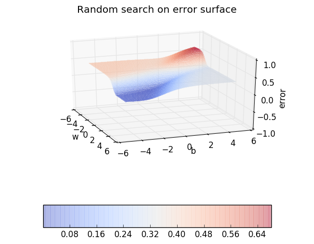
Learning Algorithm
Can we visualise this better ?
(c) One Fourth Labs
Initialise
0. Same algo as on previous slide
1. Same stuff as the previous slide except that now instead of the table we will have a 3d plot for loss v/s w,b
2. first just show the 3 axes so that I can talk through them and explain what each axes means
3. now plot the error surface (use different colors than what we use in the course, also make the surface a bit more transparent
4. now show what happens as you change the value of w,b in each iteration
\(w_1, w_2, b \)
Iterate over data:
\( \mathscr{L} = compute\_loss(x_i) \)
\( update(w_1, w_2, b, \mathscr{L}) \)
till satisfied
Learning Algorithm
What is our aim now ?
(c) One Fourth Labs
Initialise
1. Start with the same algo as on previous slide
2. Replace guess_and_update by w = w+\delat w and b = b + \delata b
3. In this box now show the plot again containing all the points and show how you were going over them one by one in the algo on LHS
4. now below this box, write \delta w= some_guess, \deltab = some_guess
\(w_1, w_2, b \)
Iterate over data:
\( \mathscr{L} = compute\_loss(x_i) \)
\( update(w_1, w_2, b, \mathscr{L}) \)
till satisfied
Show a quote here which says that
"Instead of guessing \delta w and \delta b, we need a principled way of changing w and b based on the loss function"
Learning Algorithm
Can we formulate this more mathematically ?
(c) One Fourth Labs
\(\theta = [w, b] \)
\(\Delta \theta = [\Delta w, \Delta b] \)
\( \theta_{new} = \theta + \eta . \Delta \theta \)
\(\theta\)
\(\Delta \theta\)
\( \eta . \Delta \theta \)
\( \theta_{new}\)
Instead of guessing \(\Delta w\) and\( \Delta\) b, we need a principled way of changing w and b based on the loss function
Learning Algorithm
Can we get the answer from some basic mathematics ?
(c) One Fourth Labs
\( \because \theta = [w, b] \)
\(w \rightarrow w + \eta \Delta w \)
\(b \rightarrow b + \eta \Delta b \)
\(\mathscr{L} (w) < \mathscr{L}(w +\eta \Delta w)\)
\( \mathscr{L} (b) < \mathscr{L}(b +\eta \Delta b)\)
\(\mathscr{L} ( \theta) < \mathscr{L}( \theta + \eta \Delta \theta)\)
\( f(x + \Delta x) = f(x) + f'(x)\Delta x + \frac{1}{2!}f''(x)\Delta x^2 + \frac{1}{3!}f'''(x)\Delta x^3 + \cdots \)
Taylor Series
\(\mathscr{L} (w,b) < \mathscr{L}(w +\eta \Delta w, b + \eta\Delta b )\)
\( \mathscr{L}(\theta + \Delta \theta) = \mathscr{L}(\theta) + \mathscr{L}'(\theta)\Delta \theta + \frac{1}{2!}\mathscr{L}''(\theta)\Delta \theta^2 + \frac{1}{3!}\mathscr{L}'''(\theta)\Delta \theta^3 + \cdots \)
Learning Algorithm
How does Taylor series help us to arrive at the answer ?
(c) One Fourth Labs
\(\mathscr{L}(\theta+\eta u) = \mathscr{L}(\theta) + \eta*u^T \nabla_{\theta} \mathscr{L}(\theta) + \frac{\eta^2}{2!}*u^T \nabla^2 \mathscr{L} (\theta)u + \frac{\eta^3}{3!}*....+ \frac{\eta^4}{4!}*...\)
\(= \mathscr{L}(\theta)+ \eta*u^T \nabla_{\theta}\mathscr{L}(\theta) [\eta is typically small, so \eta^2, \eta^3, ... \rightarrow 0]\)
Note that the move \( \eta u \) would be favorable only if,
\( \mathscr{L}(\theta+\eta u) - \mathscr{L}(\theta) < 0\) [ i.e. if the new loss is less than the previous loss]
This implies,
\( u^T \nabla_{\theta} \mathscr{L}(\theta) < 0 \)
For ease of notation,
let \( \Delta\theta = u\),
Then from Taylor series, we have,
Learning Algorithm
How does Taylor series help us to arrive at the answer ?
(c) One Fourth Labs
Okay, so we have,
\( u^T \nabla_{\theta} \mathscr{L}(\theta) < 0 \)
But, what is the range of \(u^T \nabla_{\theta}\mathscr{L}(\theta) \) ?
Let \(\beta\) be the angle between \(u\) and \(\nabla_{\theta}\mathscr{L}(\theta)\), then we know that,
\(-1 \leq cos(\beta) = \frac{u^T \nabla_{\theta}\mathscr{L}(\theta)}{||u||*||\nabla_{\theta}\mathscr{L}(\theta)||} \leq 1\)
multiply throughout by k = \( ||u||*||\nabla_{\theta}\mathscr{L}(\theta)||\)
\( -k \leq k*cos(\beta) = u^T \nabla_{\theta}\mathscr{L}(\theta) \leq k \)
Thus, \( \mathscr{L}(\theta + \eta u) - \mathscr{L}(\theta) = u^T \nabla_{\theta}\mathscr{L}(\theta) = k*\cos \beta \) will be most negative
when \(\cos(\beta)\) = -1 i.e., when \(\beta\) is 180\(\degree \)
Learning Algorithm
How does Taylor series help us to arrive at the answer ?
(c) One Fourth Labs
Gradient Descent Rule,
- The direction \(u\) that we intend to move in should be at \(180\degree\) w.r.t. the gradient.
- In other words, move in a direction opposite to the gradient.
Parameter Update Rule
\(w_{t+1} = w_{t} - \eta \Delta w_{t} \)
\(b_{t+1} = b_{t} - \eta \Delta b_{t} \)
\( where \Delta w_{t} =\frac{\partial \mathscr{L}(w, b)}{\partial w}_{at w = w_t, b= b_t}, \Delta b_{t} = \frac{\partial \mathscr{L}(w,b)}{\partial b}_{at w = w_t, b = b_t}\)
So we now have a more principled way of moving in the w-b plane than our "guesswork'' algorithm
Learning Algorithm
How does the algorithm look like now ?
(c) One Fourth Labs
Initialise
\(w, b \)
Iterate over data:
\(w_{t+1} = w_{t} - \eta \Delta w_{t} \)
till satisfied
How do I compute \( \Delta w\) and\( \Delta b \)?
\(b_{t+1} = b_{t} - \eta \Delta b_{t} \)
Learning Algorithm
How do I compute \(\Delta w \) and \(\Delta b\)
(c) One Fourth Labs
\(\mathscr{L} = \frac{1}{5} \sum_{i = 1}^{i=5}(f(x_i) - y_i)\)
\(\frac{\partial \mathscr{L}}{\partial w} = \frac{\partial}{\partial w}[ \frac{1}{5} \sum_{i = 1}^{i=5}(f(x_i) - y_i)]\)
\(\Delta w = \frac{\partial \mathscr{L}}{\partial w} = \frac{1}{5} \sum_{i = 1}^{i=5}\frac{\partial}{\partial w} (f(x_i) - y_i)\)
Let's consider only one term in this sum,

Learning Algorithm
How do I compute \(\Delta w \) and \(\Delta b\)
(c) One Fourth Labs
\(\nabla w = \frac{\partial}{\partial w}[\frac{1}{2}*(f(x) - y)^2] \)
\(= \frac{1}{2}*[2*(f(x) - y) * \frac{\partial}{\partial w} (f(x) - y)]\)
\(= (f(x) - y) * \frac{\partial}{\partial w}(f(x)) \)
\(= (f(x) - y) * \frac{\partial}{\partial w}\Big(\frac{1}{1 + e^{-(wx + b)}}\Big) \)
\( = \color{red}{(f(x) - y) * f(x)*(1- f(x)) *x}\)
\( \frac{\partial}{\partial w}\Big(\frac{1}{1 + e^{-(wx + b)}}\Big)\)
\( =\frac{-1}{(1 + e^{-(wx + b)})^2}\frac{\partial}{\partial w}(e^{-(wx + b)})) \)
\( =\frac{-1}{(1 + e^{-(wx + b)})^2}*(e^{-(wx + b)})\frac{\partial}{\partial w}(-(wx + b)))\)
\( =\frac{-1}{(1 + e^{-(wx + b)})}*\frac{e^{-(wx + b)}}{(1 + e^{-(wx + b)})} *(-x)\)
\( =\frac{1}{(1 + e^{-(wx + b)})}*\frac{e^{-(wx + b)}}{(1 + e^{-(wx + b)})} *(x)\)
\( =f(x)*(1- f(x))*x \)
Learning Algorithm
How do I compute \(\Delta w \) and \(\Delta b\)
(c) One Fourth Labs
\(\mathscr{L} = \frac{1}{5} \sum_{i = 1}^{i=5}(f(x_i) - y_i)\)
\(\frac{\partial \mathscr{L}}{\partial w} = \frac{\partial}{\partial w}[ \frac{1}{5} \sum_{i = 1}^{i=5}(f(x_i) - y_i)]\)
\(\Delta w = \frac{\partial \mathscr{L}}{\partial w} = \frac{1}{5} \sum_{i = 1}^{i=5}\frac{\partial}{\partial w} (f(x_i) - y_i)\)
Let's consider only one term in this sum,
\(\Delta w=(f(x) - y) * f(x)*(1- f(x)) *x \)
For 5 points,
\(\Delta w=\sum_{i=1}^{i=5} (f(x_i) - y_i) *f(x_i))*(1- f(x_i)) *x_i \)
\(\Delta b=\sum_{i=1}^{i=5} (f(x_i) - y_i) * f(x_i))*(1- f(x_i)) \)
Learning Algorithm
How do I compute \(\Delta w \) and \(\Delta b\)
(c) One Fourth Labs
\(\mathscr{L} = \frac{1}{2} \sum_{i = 1}^{i=5}(f(x_i) - y_i)\)
\(\frac{\partial \mathscr{L}}{\partial w} = \frac{\partial}{\partial w}[ \frac{1}{2} \sum_{i = 1}^{i=5}(f(x_i) - y_i)]\)
\(\Delta w = \frac{\partial \mathscr{L}}{\partial w} = \frac{1}{2} \sum_{i = 1}^{i=5}\frac{\partial}{\partial w} (f(x_i) - y_i)\)
Let's consider only one term in this sum
\(\Delta w=(f(x) - y) * f(x)*(1- f(x)) *x \)
For 5 points,
\(\Delta w=\sum_{i=1}^{i=5} (f(x_i) - y_i) *f(x_i))*(1- f(x_i)) *x_i \)
\(\Delta b=\sum_{i=1}^{i=5} (f(x_i) - y_i) * f(x_i))*(1- f(x_i)) \)
Learning Algorithm
How does the full algorithm look like ?
(c) One Fourth Labs
Learning Algorithm
What happens when we have more than 2 parameters ?
(c) One Fourth Labs
1. Show a dataset containing 5 input variables
2. Show the corresponding model equation
3. Now show the algorithm from before but now instead of update rules for w and b you will have update rules for w_1,...w_5 and b
4. Now show the equation for \delta_w and \delta_b from before
5. Now replace w by w_1 and x by x_1 in the formula for dL/dw (on the next slide have the full derivation)
6. Now say that in general dL/dw_1 = ....
Learning Algorithm
What happens when we have more than 2 parameters ?
(c) One Fourth Labs
Show the full derivation for dL/dw_1
Learning Algorithm
What happens when we have more than 2 parameters ?
(c) One Fourth Labs
Now take the slide 8.5 and modify it so that you have gradient descent code for 5 variables (the code has to be modularized and generalized for k variables)
It would be great if we can then convert the above code to vector form where we directly do everything in terms of \theta where \theta = [w1, w2, w3, w4, w5]
Now run the code and on the RHS show a plot of how the loss decreases with number of iterations
Evaluation
How do you check the performance of the sigmoid model?
(c) One Fourth Labs
Same slide as that in MP neuron
Take-aways
What are the new things that we learned in this module ?
(c) One Fourth Labs
Show the 6 jars at the top (again can be small)
\( \{0, 1\} \)
\( \in \mathbb{R} \)
Tasks with Real inputs and real outputs
show the sigmoid plot with the issue of non-linearly separable data
show squared error loss
show gradient descent update rule
show accuracy formula
Take-aways
What are the new things that we learned in this module ?
(c) One Fourth Labs
A slide where we compare sigmoid, perceptron and MP neuron in terms of 6 jars
Still not complex enough to handle non-linear data
Copy of jaya's copy of 1.7 Sigmoid Neuron
By Shubham Patel


