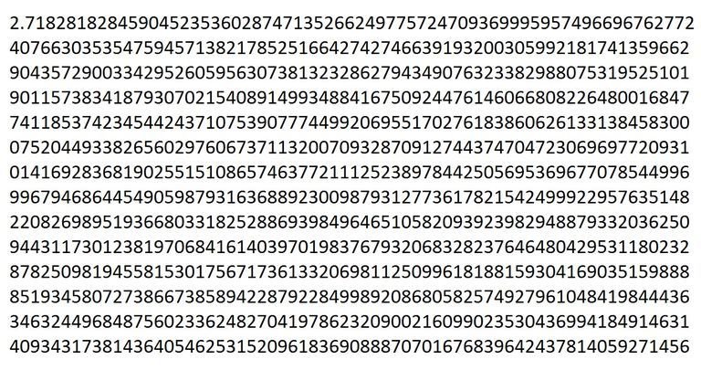
Lost in Mathematical constant(e), Python to rescue


SHWETA SUMAN
cosmologist10.github.io
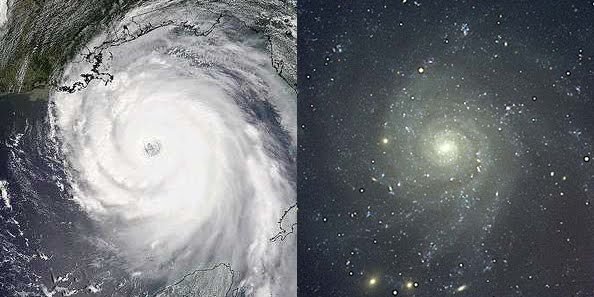
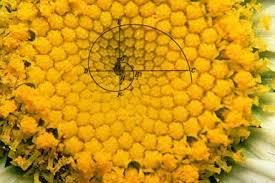
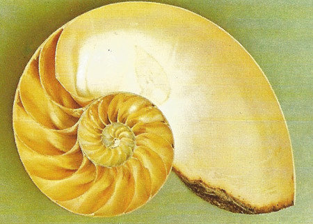
Logarithmic Spirals
Coordinate System
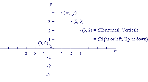
Rectangular
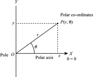
Polar
Bernoulli’s equation to define logarithmic spirals, in polar coordinates :
lnr = aθ
r = e^(aθ)
x, y = r cosθ, r sinθ
import matplotlib as mpl
from mpl_toolkits.mplot3d import Axes3D
import numpy as np
import matplotlib.pyplot as plt
from math import exp,sin,cos
from pylab import *
import argparse

def LogarithmicSpirals(constant) :
    """ Calculates the radius, values of x and y co-ordinates and plot it ."""

    theta = np.linspace(0, 500, 10000) # theta
    radius = exp(constant*theta) # calculate radius
    # Get the x and y coordinates
    x = radius*cos(theta)
    y = radius*sin(theta)
    ax.plot(x, y)
    ax.legend()
    plt.show()

if __name__ ==  "__main__":
    parser = argparse.ArgumentParser(prog='logarithmspirals', description='Logarithmic Spirals')
    parser.add_argument('-C','--constant',help='Constant',type=float, default=0.05)
    args = parser.parse_args()

    mpl.rcParams['legend.fontsize'] = 10
    fig = plt.figure()
    ax = fig.gca(projection='3d')

    LogarithmicSpirals(args.constant)
Draw logarithmic spiral
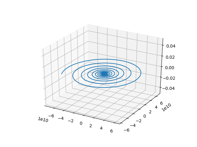
Plotted graph
To analyze the common properties, plotted the graph in 2d and used annotations.
from math import exp
import numpy as np
import matplotlib.pyplot as plt

theta = np.linspace(0, 500, 10000)
a = 0.05
fig = plt.figure()
ax = fig.add_subplot(111, polar=True)
r = np.exp(0.05*theta)
line, = ax.plot(theta, r, color='#ee8d18', lw=3)

ind = 800
thisr, thistheta = r[ind], theta[ind]
ax.plot([thistheta], [thisr], 'o')

ax.annotate('a polar annotation',
            xy=(thistheta, thisr),  # theta, radius
            xytext=(0.05, 0.05),    # fraction, fraction
            textcoords='figure fraction',
            horizontalalignment='left',
            verticalalignment='bottom',
            )
plt.show()
Properties :
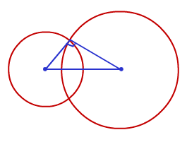
- Every straight line through the center intersects the spiral at the exact same angle (In fact Circle is a logarithmic spiral whose angle of intersection is 90 degree and rate of growth is 0).
- Rotating the spiral by equal amount increases the distance from center by In fact ratios, that is, in a geometric progression.
An angle of Intersection of Circle
Rotation of Spirals
e^x: The Function That Equals Its Own Derivative

Rate of decay of Radioactive substance
m = mₐe^(-a*t)
amount of radiation a radioactive substance proportional to mass
mₐ =initial mass of the substance(where t = 0)
a = rate of decay of substance, measured by half-life
from scipy.optimize import curve_fit
import numpy as np
from matplotlib import pyplot as plt

# define type of function to search
def model_func(t, m, a, b):
    return m * np.exp(-a*t) + b

# sample data
x = np.array([399.75, 989.25, 1578.75, 2168.25, 2757.75, 3347.25, 3936.75, 4526.25, 5115.75, 5705.25])
y = np.array([109,62,39,13,10,4,2,0,1,2])

# curve fit
p0 = (1.,1.e-5,1.) # starting search koefs
opt, pcov = curve_fit(model_func, x, y, p0)
a, k, b = opt

# test result
x2 = np.linspace(250, 6000, 250)
y2 = model_func(x2, a, k, b)
fig, ax = plt.subplots()
ax.plot(x2, y2, color='r', label='Fit. func: $f(x) = %.3f e^{%.3f x} %+.3f$' % (a,k,b))
ax.plot(x, y, 'bo', label='data with noise')
ax.legend(loc='best')
plt.show()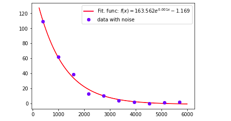
Sound wave travel through air
I= Ioe^(-ax)
I = Intensity
differential equation dI/dx = -aI,
where x is the distance traveled
x = Distance travelled
graph of (e^x + e^-x)
x = np.linspace(-2, 2, 10000)
y = (np.exp(x) + np.exp(-x))
plt.figure()
plt.plot(x, y)
plt.xlabel('$x$')
plt.ylabel('$\exp(x)+exp(-x)$')
plt.show()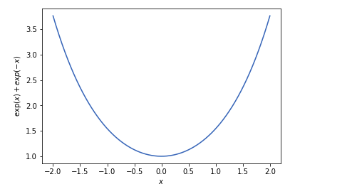
cosh x
graph of (e^x + e^-x)
x = np.linspace(-2, 2, 10000)
y = (np.exp(x) - np.exp(-x))
plt.figure()
plt.plot(x, y)
plt.xlabel('$x$')
plt.ylabel('$\exp(x)-exp(-x)$')
plt.show()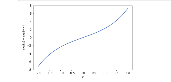
Calculus
Algebra
Geometry
All on the same page
(Rate of change)
Geometric progression
Hyperbola
Origination of e
Question of Finance
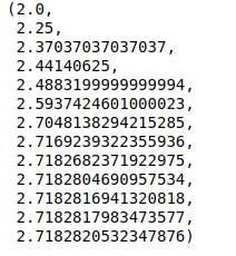
An account starts with $1.00 and pays 100 percent interest per year. If the interest is credited once, at the end of the year, the value of the account at year-end will be $2.00. What happens if the interest is computed and credited more frequently during the year?
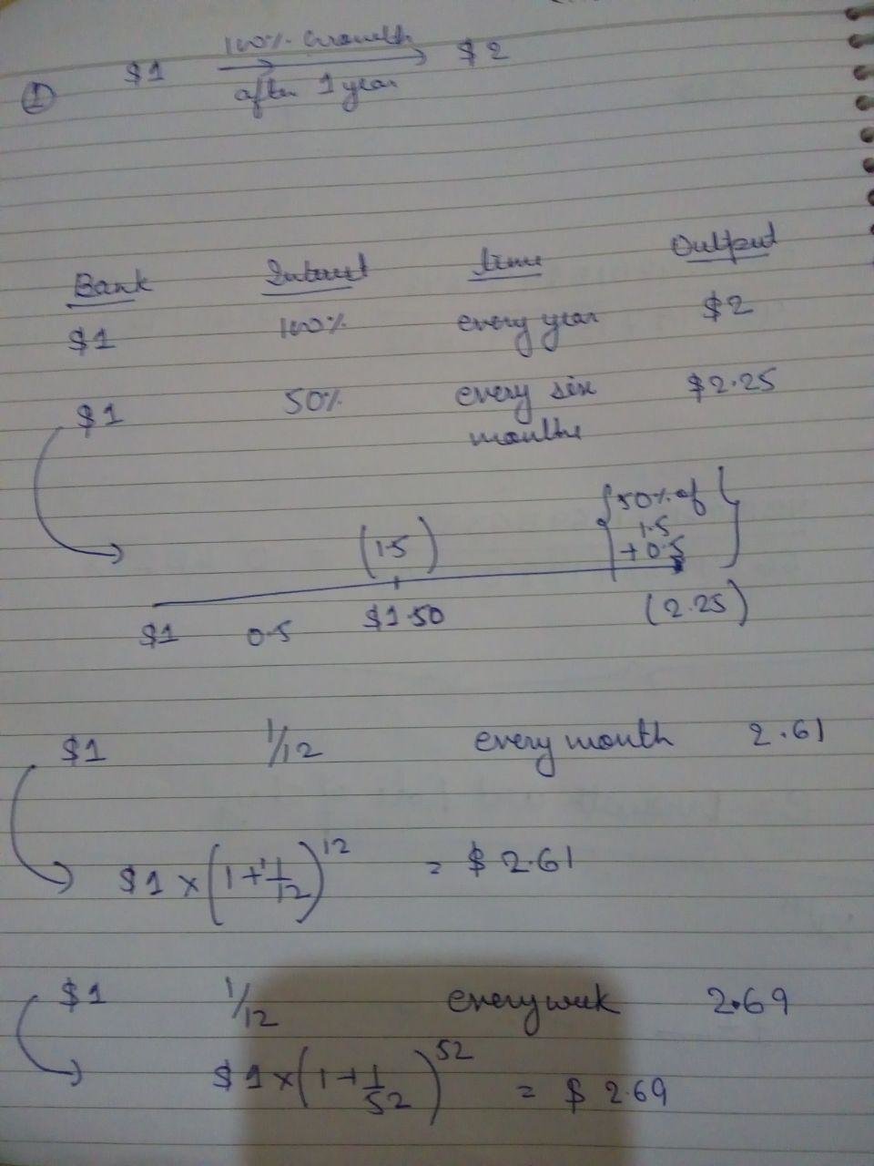
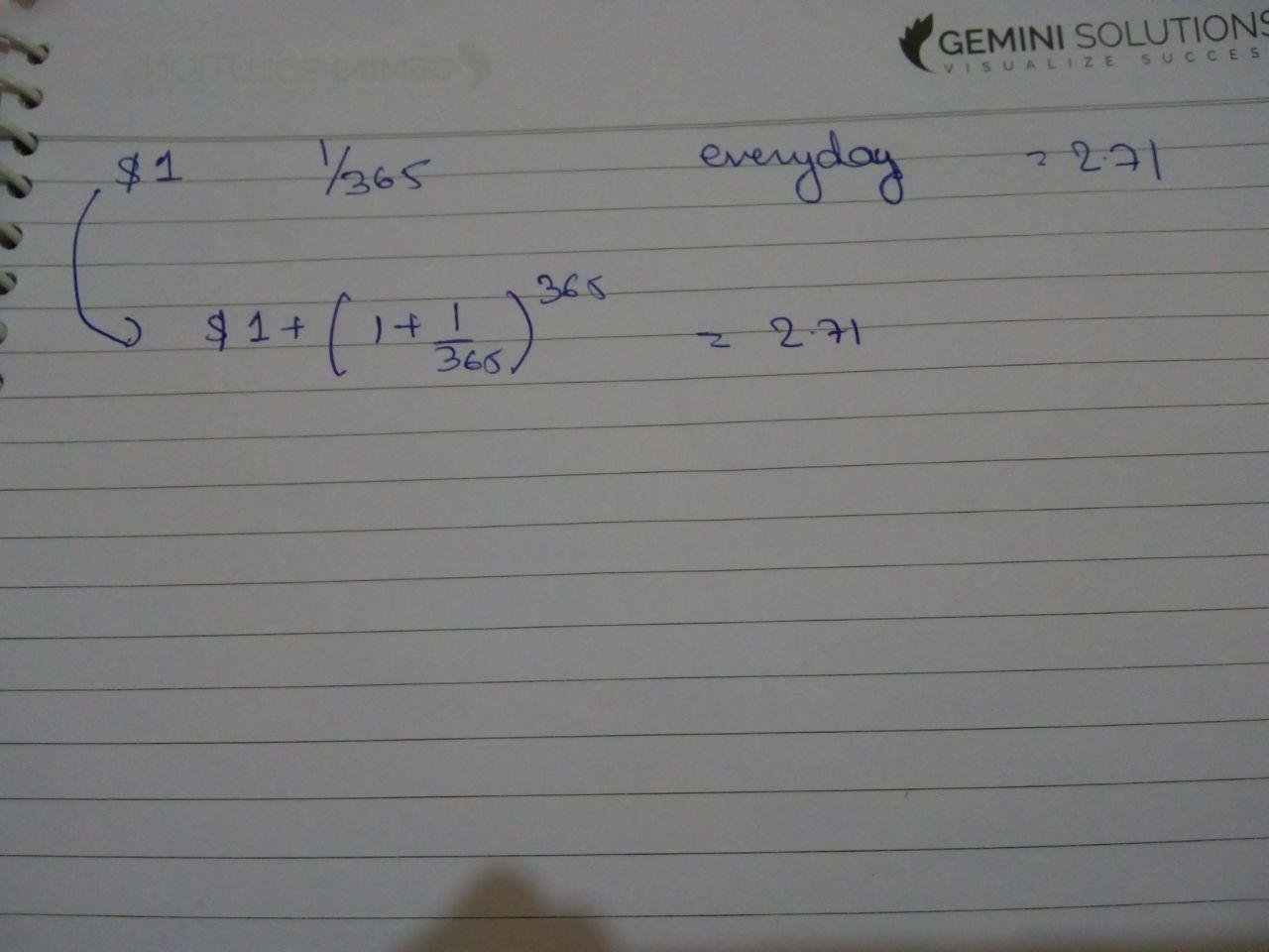
$1.00×(1 + 1/n)n = (1 + 1/n)n
def cal_fin(n):
    return (1 + 1/n)**n

cal_fin(1),cal_fin(2),cal_fin(3),cal_fin(4),cal_fin(5),cal_fin(10),
cal_fin(100),cal_fin(1000),cal_fin(100000),cal_fin(1000000),
cal_fin(10000000),cal_fin(100000000),cal_fin(10000000000),
Forefathers of the Calculus
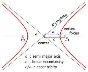
Hyperbola
Infinite sum series
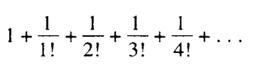

from tco import *
@with_continuations()
def factorial(n, k, self=None):
    return self(n-1, k*n) if n > 1 else k

def calc(u):
    return sum([1.0/factorial(i, 1) for i in range(0, u+1)])
The Famous of All formulas
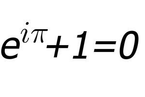
Thanks for listening!
Shweta Suman
sumanshweta44@gmail.com
deck
By shweta suman


