COMP2521
Data Structures & Algorithms
Week 2.1
Performance Analysis
Author: Hayden Smith 2021
In this lecture
Why?
- Understanding the time and storage demands of different data structures and algorithms is critical in writing the right code for a program
What?
- Data Structures
- Algorithms
- Pseudocode
- Time Complexity
- Space Complexity
Measuring Literal Program Run Time
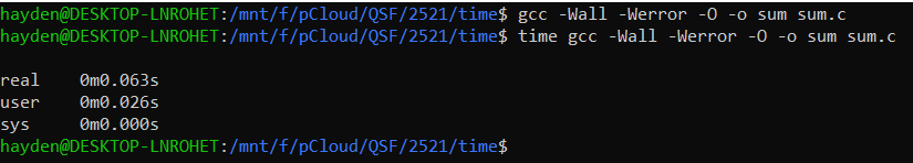
For any linux command or program, we can measure the time it takes to run. We simply add time to the front of the command.
- real: time taken on the clock to complete
- user: time taken for the CPU to process your program
- sys: time taken by the operating system for special actions (e.g. malloc, file open & close)
Analysing a "sum" program
We have a simple program sum.c that reads numbers in from STDIN, and produces a sum. We also have some test files.
#include <stdio.h>

int main(int argc, char* argv[]) {
    int temp;
    int sum = 0;
    while (scanf("%d", &temp) != -1) {
        sum += temp;
    }
    printf("%d\n", sum);
    return 0;
}
- sum100000.txt: 100,000 numbers
- sum1000000.txt: 1,000,000 numbers
- sum10000000.txt: 10,000,000 numbers
- sum100000000.txt: 100,000,000 numbers
- sum1000000000.txt: 1,000,000,000 numbers
sum.c
$ gcc -Wall -Werror -o sum sum.c
$ time ./sum < sum10000.txt
Can we run and plot the results? How would you describe how long this program takes? How does the time taken change with the changing size of input?
How much memory does this program use when running? How does the memory change with the changing size of input?
Analysing a "sum" program
Analysing a "sort" program
We have a simple program sort.c that reads numbers in from STDIN, and produces those numbers in sorted order. It uses a bubble sort. We also have some test files. Can we run and plot the results?
| numbers | sorted file | reverse sorted file | random file |
|---|---|---|---|
| 100 | sorted100.txt | rev_sorted100.txt | random100.txt |
| 1000 | sorted1000.txt | rev_sorted1000.txt | random1000.txt |
| 5000 | sorted5000.txt | rev_sorted5000.txt | random5000.txt |
| 10000 | sorted10000.txt | rev_sorted10000.txt | random10000.txt |
| 50000 | sorted50000.txt | rev_sorted50000.txt | random50000.txt |
| 100000 | sorted100000.txt | rev_sorted100000.txt | random100000.txt |
How do we even sort numbers??
Firstly, let's understand the sort. One of the simplest ways to sort numbers is known as a bubble sort.
#define TRUE 1
#define FALSE 0

void sort(int *nums, int size) {
    int sorted = FALSE;
    while (sorted == FALSE) {
        sorted = TRUE;
        for (int i = 0; i < size - 1; i++) {
            if (nums[i] > nums[i + 1]) {
                int temp = nums[i];
                nums[i] = nums[i + 1];
                nums[i + 1] = temp;
                sorted = FALSE;
            }
        }
    }
}
A bubble sort
Can we run and plot the results? How would you describe how long this program takes? How does the time taken change with the changing size of input?
How much memory does this program use when running? How does the memory change with the changing size of input?
Analysing a "sort" program
Using the "time" command and looking at RAM usage has it's issues when trying to understand general program behaviour:
- Requires implementation of the algorithm
- Running time is easily influenced by specific machine
- Need to use same machine and circumstances to compare different algorithms
We need a way of theoretically analysing an algorithm, and a non-C language to do this in.
Issues with literal program run-time
Pseudocode
Pseudocode is a method of describing the behaviour of a program without needing to worry about the language it's written in or the machine it runs on.
- More structured than English
- Less structured than code
Pseudocode
#include <stdio.h>

int main(int argc, char* argv[]) {
    int temp;
    int sum = 0;
    while (scanf("%d", &temp) != -1) {
        sum += temp;
    }
    printf("%d\n", sum);
    return 0;
}
sum.c
#include <stdio.h>

int main(int argc, char* argv[]) {
    int temp;
    int sum = 0;
    while (scanf("%d", &temp) != -1) {
        sum += temp;
    }
    printf("%d\n", sum);
    return 0;
}
sum psuedocode
function sumNumbers() {
    sum = 0
    while (read number from STDIN as "i") {
        sum += i
    }
    print(sum)
}
Pseudocode
#include <stdio.h>

int main(int argc, char* argv[]) {
    int temp;
    int sum = 0;
    while (scanf("%d", &temp) != -1) {
        sum += temp;
    }
    printf("%d\n", sum);
    return 0;
}
sum.c
#include <stdio.h>

int main(int argc, char* argv[]) {
    int temp;
    int sum = 0;
    while (scanf("%d", &temp) != -1) {
        sum += temp;
    }
    printf("%d\n", sum);
    return 0;
}
sum psuedocode
begin sumNumbers:
    sum = 0
    foreach number from STDIN:
        sum += (number read in)
    print sum
Pseudocode
#include <stdio.h>

int main(int argc, char* argv[]) {
    int temp;
    int sum = 0;
    while (scanf("%d", &temp) != -1) {
        sum += temp;
    }
    printf("%d\n", sum);
    return 0;
}
sort.c
#define TRUE 1
#define FALSE 0

void sort(int *nums, int size) {
    int sorted = FALSE;
    while (sorted == FALSE) {
        sorted = TRUE;
        for (int i = 0; i < size - 1; i++) {
            if (nums[i] > nums[i + 1]) {
                int temp = nums[i];
                nums[i] = nums[i + 1];
                nums[i + 1] = temp;
                sorted = FALSE;
            }
        }
    }
}
sort psuedocode
begin sort(list):
    sorted = false
    while not sorted:
        sorted = true
        for all elements of list:
            if list[i] > list[i + 1]:
                swap(list[i], list[i + 1])
    return list
Theoretical Performance Analysis
If we look at the pseudocode of a program, we can evaluate it's complexity regardless of the hardware or software environment.
For time complexity, we do this by counting how many "operations" occur in a program. Then we express the complexity of the program as an equation based on a variable "n" where "n" is the number of input elements.
Analysing a simple program
Do an analysis on each line. Mostly you can just count each line independently, as we can generally assume a line has a single unit cost of work.
When you enter a loop you have to multiply the cost of the line by the number of times it's being looped.
For some algorithms you can analyse it for best case and worst case input (and sometimes these are the same).
Analysing a simple program
begin sort(list):
    sorted = false                          | 1         | 1
    while not sorted:                       | n         | n
        sorted = true                       | * 1       | n * 1
        for all elements of list:           | * n       | n * n
            if list[i] > list[i + 1]:       |   * 1     | n * n * 1
                swap(list[i], list[i + 1])  |   * 1     | n * n * 1
                sorted = false              |   * 1     | n * n * 1
    return list                             | 1         | 1
--------------------------------------------------------------------
                                     1 + n + n + n^2 + n^2 + n^2 + n^2 + 1
                                  =  4n^2 + 2n + 2
bubble sort: worst case (numbers reverse sorted)
- Time complexity: 4n^2 + 2n + 2
- Space complexity: 1
Analysing a simple program
begin sort(list):
    sorted = false                          | 1         | 1
    while not sorted:                       | n         | n
        sorted = true                       | * 1       | n * 1
        for all elements of list:           | * 1       | n * 1
            if list[i] > list[i + 1]:       |   * 0     | n * 1 * 0
                swap(list[i], list[i + 1])  |   * 0     | n * 1 * 0
                sorted = false              |   * 0     | n * 1 * 0
    return list                             | 1         | 1
--------------------------------------------------------------------
                                              1 + n + n + n + 1
                                           =  3n + 2
bubble sort: best case (numbers sorted)
- Time complexity: 3n + 2
- Space complexity: 1
Analysing a simple program
function sumNumbers():                      |
    sum = 0                                 | 1
    while (read number from STDIN as "i"):  | n
        sum += i                            | * 1
    print(sum)                              | 1
--------------------------------------------------------------------
                                              1 + n + n + 1
                                            = 2n + 2
Best and worst case are the same
- Time complexity: 2n + 2
- Space complexity: 1
Primitive Operations
We usually assume that primitive operations are "constant time" (i.e. are just 1 step of processing). In reality they might be one step, or a few steps, but as we'll see soon it doesn't matter.
Primitive operations include:
- Indexing an array (getting or setting)
- Comparisons (equality, relational)
- Variable assignment
Big-O Notation
As discussed, we can write a mathematical expression (in terms of something like "n", the number of inputs) to generalise how much time or space a program needs.
However, to simplify this further, we:
- Remove any constant factors in front of variables
- Remove any lower order variables
This produces a program's Big-O number. E.G. O(n^2)
Big-O Notation
| General Complexity | Big-O Value |
|---|---|
| n^2 | O(n^2) |
| 3n | O(n) |
| 3n + 3 | O(n) |
| 2n^2 + 4n - 5 | O(n^2) |
| 3n*log(n) | O(n*log(n)) |
| log(n) + 2 | O(log(n)) |
| n + log(n) | O(n) |
| n^2 + n + log(n) | O(n^2) |
Big-O Notation
Generally speaking your Big-O will be a product or single of any of these base complexities:
- Constant ≅ 1
- Logarithmic ≅ log n
- Linear ≅ n
- N-Log-N ≅ n log n
- Quadratic ≅ n2
- Cubic ≅ n3
- Exponential ≅ 2n
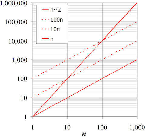
Why remove things?
Factors and lower orders are removed because they become irrelevant at scale.
Most of the time, programs that operate on small numbers finish extremely quickly (computers can process hundreds of millions of operations per second). Therefore our focus is on the general behaviour of programs for large inputs.
Why remove things?
Why is an 2n^2 + 1000 program O(n^2)?
| n | n^2 | 2n^2 | 2n^2 + 1000 |
|---|---|---|---|
| 10 | 100 (fast) | 200 (fast) | 2,000 (fast) |
| 100 | 10,000 (fast) | 20,000 (fast) | 101,000 (fast) |
| 1,000 | 1,000,000 (5ms) | 2,000,000 (10ms) | 10,001,000 (10ms) |
| 10,000 | 100,000,000 (0.5 sec) | 200,000,000 (1 sec) | 200,001,000 (1 sec) |
| 100,000 | 100,000,000,000 (8 min) | 200,000,001,000 (16 min) | 200,000,001,000 (16 min) |
| 1,000,000 | 1,000,000,000,000 (1.3 hours) | 2,000,000,000,000 (2.6 hours) | 2,000,000,001,000 (2.6 hours) |
Because for large n, n^2 dominates the other components
Why remove things?
Analysing a "search" program
We have a simple program search.c that reads numbers in from STDIN, and then reads one final number which is the number to search for. It then prints whether it was found or not.
Analysing a "search" program
We have a simple program search.c that reads numbers in from STDIN, and then reads one final number which is the number to search for. It then prints whether it was found or not.
function searchLinear(array, lookingFor):
    for each element in array:
        if element == lookingFor:
            return true
    return false
function searchBinary(array, lookingFor):
leftBound = 0
rightBound = size of array
guessIndex = (rightBound + leftBound) / 2
loop until found:
if array[guessIndex] < lookingFor:
leftBound = guessIndex
guessIndex = (rightBound + leftBound) / 2
else if array[guessIndex] > lookingFor:
rightBound = guessIndex
guessIndex = (rightBound + leftBound) / 2
else:
return true
linear search
binary search (only for sorted)
Analysing a "search" program
Let's discuss the time complexities of these two different approaches.
Amortisation
Amorisation: In simple terms, it is the process of doing some work up front, to reduce the work later on.
What are examples of this in real life?
How do we apply this to thinking about the problems in this lecture?
Summary of complexities
Time Complexity
| Program | Best Case | Worst Case | Average Case |
|---|---|---|---|
| sum.c | O(n) | O(n) | O(n) |
| sort.c | O(n) | O(n^2) | O(1/2*n^2) = O(n^2) |
| search.c (binary) | log(n)* | log(n)* | log(n)* |
| search.c (standard) | O(1) | O(n) | O(1/2*n) = O(n) |
Space Complexity
| Program | Best Case | Worst Case | Average Case |
|---|---|---|---|
| sum.c | O(1) | O(1) | O(1) |
| sort.c | O(1) | O(1) | O(1) |
| search.c (binary) | O(1) | O(1) | O(1) |
| search.c (standard) | O(1) | O(1) | O(1) |
* Binary search is log(n) assuming the numbers are sorted. Sorting the numbers might be n^2, which is negligable if you only have to sort them once for MANY searches. If you have to sort them for one search then a standard search is better.
Copy of COMP2521 21T2 - 2.1 - Performance Analysis
By Sim Mautner


