Significance Tests for Feature Relevance of a Black-Box Learner

DOI: 10.1109/TNNLS.2022.3185742

DOC: dnn-inference.readthedocs.io

(Joint work with Xiaotong Shen and Wei Pan)

Ben Dai (CUHK)

Illustrative Results

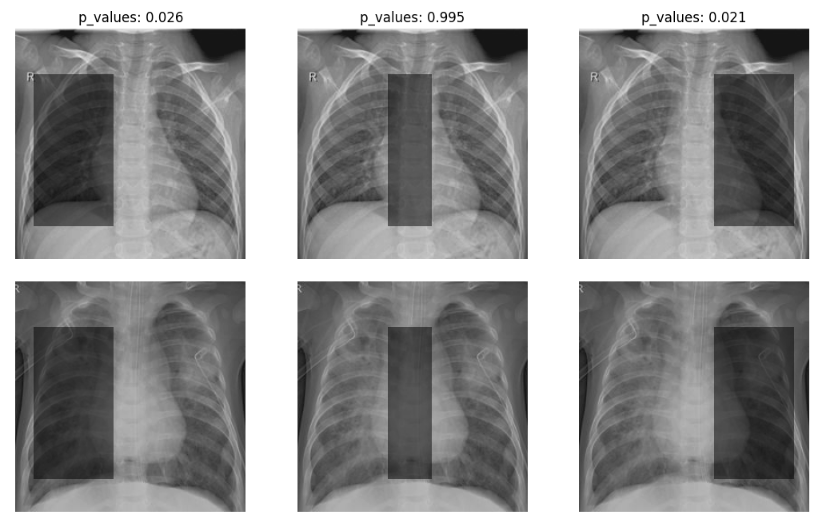
p-values for significance of keypoints to facial expression recognition based on the VGG neural network.

Application:

• facilitate visual-based decision-making
• provide instructive information for visual sensor management and construction.

Motivation

• Question: Can we provide a  valid p-value  for any pre-specified region (features) based on a black-box model, such as a DL model?

• Why significance tests? Hypothesis testing, feature interpretation, XAI, make black-box models more reliable ...

• Why region tests? For image analysis, the impact of each pixel is negligible but a pattern of a collection of pixels (e.g. a region) may instead become salient.

• Why black-box models? Significant improvement in prediction performance, which enforce us to believe that a black-box model is a better option to model real data. For example, use a CNN to formulate image data.

Difficulty

• Black-box models. It is infeasible (or difficult) to ``open the box'', that is, we only access the input and output for a black-box model, and do not know its inner structure.
  • Feature-param correspondence. The feature-parameter correspondence is unclear for black-box models, such as CNNs and RNNs.

Difficulty

He, K. et al. (2015) Deep residual learning for image recognition. CVPR.

Difficulty

• Black-box models. It is infeasible (or difficult) to ``open the box'', that is, we only access the input and output for a black-box model, and do not know its inner structure.
  • Feature-param correspondence. The feature-parameter correspondence is unclear for black-box models, such as CNNs and RNNs.
• High-dimensional hypothesized features. The dimension of the hypothesized features could be extremely large.
• Computationally expensive. Refitting a deep learning model is computationally expensive.

• Overparametrized models. When the number of parameters increase, both training / testing errors decrease, and the training error could be zero.

Neyshabur, B., Li, Z., Bhojanapalli, S., LeCun, Y., & Srebro, N. (2018). Towards understanding the role of over-parametrization in generalization of neural networks.

Issues of Existing Methods

• Likelihood Ratio Test (LRT)
  • black-box models and overparam. Taylor expansion is infeasible, and the training loss could be very small.
  • Feature-param.  LRT works for \(\mathbf{\theta} \in \mathbf{\Theta} \ \text{vs} \ \mathbf{\theta} \notin \mathbf{\Theta}\)

• Conditional randomization test (CRT; Candes et al. 2018) and holdout randomization test (HRT; Tansey et al. 2018)

  • significance testing for a single feature.

  • require conditional Prob of hypothesized feature given the others. It is usually difficult to estimate for complex datasets.

• Leave-one-covariate-out (LOCO; Lei et al. 2018)

  • significance testing for a single feature.

  • finite-sample hypothesis testing.

Goodness

• Dataset \((\mathbf{X}_i, \mathbf{Y}_i)_{i=1}^N\)

  • Input and output \(\mathbf{X}_{i} \in \mathbb{R}^d; \mathbf{Y}_{i} \in \mathbb{R}^K\)
  • large-scale dataset: \(N\) is large

• Black-box model \( f: \mathbb{R}^d \to \mathbb{R}^K \)

  • good performance, or small generalization error, or reasonable convergence rate

• Flexible computing platforms for a general loss function \(l(\cdot, \cdot)\)

  • TensorFlow, Keras, Pytorch

Goodness

Tan, M., & Le, Q. (2019). Efficientnet: Rethinking model scaling for convolutional neural networks. ICML, PMLR.

Proposed Hypothesis

• Goal. testing the relevance of a sub-feature \( \mathbf{X}_{\mathcal{S}} = \{ X_j; j \in \mathcal{S} \} \) to the outcome \(\mathbf{Y}\) without specifying any form of the pred function, where \(\mathcal{S}\) is an index set of hypothesized features.

• Hypothesis for feature relevance. One of the most frequently used hypothesis is conditional independence.

$$H_0: \ \bm{Y} \perp \bm{X}_\mathcal{S} \mid \bm{X}_{\mathcal{S}^c}$$

(Sometimes, people think that it is too strong.)

Proposed Hypothesis

• Goal. testing the relevance of a sub-feature \( \mathbf{X}_{\mathcal{S}} = \{ X_j; j \in \mathcal{S} \} \) to the outcome \(\mathbf{Y}\) without specifying any form of the pred function, where \(\mathcal{S}\) is an index set of hypothesized features.
• Our null/alternative Hypothesis: directly compare perf w/- or w/o hypothesized features
  • dual data \((\mathbf{Z}, \mathbf{Y})\), with permutation of \(\mathbf{X}_{\mathcal{S}}\), and \(\mathbf{Z}_{\mathcal{S}^c} = \mathbf{X}_{\mathcal{S}^c}\).
  • Risk functions. $$R(f) = \mathbb{E}\big(l(f(\bm{X}), \bm{Y}) \big), \quad R_\mathcal{S}(g) = \mathbb{E}\big(l(g(\bm{Z}), \bm{Y}) \big)$$
  • Population minimizer $$f^*=\text{argmin}_{f} R(f), \quad g^*=\text{argmin}_{g} R_\mathcal{S}(g)$$

Proposed Hypothesis

$$H_0: R(f^*)- R_\mathcal{S}(g^*)=0, \text{ versus } H_a: R(f^*) - R_\mathcal{S}(g^*)<0.$$

Best prediction based on \(\mathbf{X}\)

Proposed Hypothesis

$$H_0: R(f^*)- R_\mathcal{S}(g^*)=0, \text{ versus } H_a: R(f^*) - R_\mathcal{S}(g^*)<0.$$

Best prediction based on \(\mathbf{X}\)

Best prediction based on \(\mathbf{X}_{\mathcal{S}^c}\)

Proposed Hypothesis

Relationships among the proposed hypothesis,and conditional independence;

$$\ \bm{Y} \perp \bm{X}_\mathcal{S} \mid \bm{X}_{\mathcal{S}^c}$$

Lemma 1 (Dai et al. 2022). For any loss function, conditional independent implies risk invariance, or

$$\bm{Y} \perp \bm{X}_\mathcal{S} \mid \bm{X}_{\mathcal{S}^c} \ \Longrightarrow \ R(f^*) - R_{\mathcal{S}}(g^*) = 0.$$

Moreover, if the negative log-likelihood is used, then \(H_0\) is equivalent to conditional independence almost surely:

$$\bm{Y} \perp \bm{X}_\mathcal{S} \mid \bm{X}_{\mathcal{S}^c}  \iff R(f^*) - R_{\mathcal{S}}(g^*) = 0.$$

Proposed Tests

• Recall the proposed hypothesis $$H_0: R(f^*)- R_\mathcal{S}(g^*)=0, \text{ versus } H_a: R(f^*) - R_\mathcal{S}(g^*)<0.$$
• Empirically { estimate (\( f^*, g^*\)), evaluate (\(R\), \(R_{\mathcal{S}}\)) }.

Zhang et al. 2017: Deep neural networks easily fit shuffled pixels, random pixels.

Question: do we need to split data? Yes!

• training loss converge to zero under random pixels, yet the testing loss is still sensible.

• Theoretically, it is not easy to find a limiting distribution based on a black-box model.

Proposed Tests

• Splitting the full dataset into estimation and inference sets and generate dual datasets

$$(\bm{X}_i, \bm{Y}_i)_{i=1}^N$$

$$(\bm{X}_i, \bm{Y}_i)_{i=1}^n$$

$$(\bm{X}_{n+j}, \bm{Y}_{n+j})_{j=1}^m$$

Proposed Tests

• Splitting the full dataset into estimation and inference sets and generate dual datasets

$$(\bm{X}_i, \bm{Y}_i)_{i=1}^N$$

$$(\bm{X}_i, \bm{Y}_i)_{i=1}^n$$

$$(\bm{X}_{n+j}, \bm{Y}_{n+j})_{j=1}^m$$

$$(\bm{Z}_i, \bm{Y}_i)_{i=1}^n$$

$$(\bm{Z}_{n+j}, \bm{Y}_{n+j})_{j=1}^m$$

Proposed Tests

• Splitting the full dataset into estimation and inference sets and generate dual datasets

$$(\bm{X}_i, \bm{Y}_i)_{i=1}^N$$

$$(\bm{X}_i, \bm{Y}_i)_{i=1}^n$$

$$(\bm{X}_{n+j}, \bm{Y}_{n+j})_{j=1}^m$$

$$(\bm{Z}_i, \bm{Y}_i)_{i=1}^n$$

$$(\bm{Z}_{n+j}, \bm{Y}_{n+j})_{j=1}^m$$

• Obtain estimator \((\widehat{f}_n, \widehat{g}_n)\) based on the estimation set, then evaluate them on the inference set:

$$\widehat{R}( \widehat{f}_n ) - \widehat{R}_{\mathcal{S}}( \widehat{g}_n )$$

Proposed Tests

• Splitting the full dataset into estimation and inference sets and generate dual datasets

$$(\bm{X}_i, \bm{Y}_i)_{i=1}^N$$

$$(\bm{X}_i, \bm{Y}_i)_{i=1}^n$$

$$(\bm{X}_{n+j}, \bm{Y}_{n+j})_{j=1}^m$$

$$(\bm{Z}_i, \bm{Y}_i)_{i=1}^n$$

$$(\bm{Z}_{n+j}, \bm{Y}_{n+j})_{j=1}^m$$

• Obtain estimator \((\widehat{f}_n, \widehat{g}_n)\) based on the estimation set, then evaluate them on the inference set:

$$\widehat{R}( \widehat{f}_n ) - \widehat{R}_{\mathcal{S}}( \widehat{g}_n )$$

Proposed Tests

• Splitting the full dataset into estimation and inference sets and generate dual datasets

$$(\bm{X}_i, \bm{Y}_i)_{i=1}^N$$

$$(\bm{X}_i, \bm{Y}_i)_{i=1}^n$$

$$(\bm{X}_{n+j}, \bm{Y}_{n+j})_{j=1}^m$$

$$(\bm{Z}_i, \bm{Y}_i)_{i=1}^n$$

$$(\bm{Z}_{n+j}, \bm{Y}_{n+j})_{j=1}^m$$

• Obtain estimator \((\widehat{f}_n, \widehat{g}_n)\) based on the estimation set, then evaluate them on the inference set:

$$\widehat{R}( \widehat{f}_n ) - \widehat{R}_{\mathcal{S}}( \widehat{g}_n )$$

Question:

• Does it provide an good estimation of \(R(f^*) - R_{\mathcal{S}}(g^*)\)?
• How about the asymptotic null distribution?

Proposed Tests

• Compare Emp \(\widehat{R}( \widehat{f}_n ) - \widehat{R}_{\mathcal{S}}( \widehat{g}_n )\) with Pop \(R( f^* ) - R_{\mathcal{S}}( g^* )\)

• Consider the following decomposition

\( \widehat{R}( \widehat{f}_n ) - \widehat{R}_{\mathcal{S}}( \widehat{g}_n) = \widehat{R}( \widehat{f}_n ) - R( \widehat{f}_n ) + R_\mathcal{S}(\widehat{g}_n) - \widehat{R}_{\mathcal{S}}( \widehat{g}_n )\)

$$+R( \widehat{f}_n ) - R( f^* ) + R_\mathcal{S}(g^*) - R_\mathcal{S}(\widehat{g}_n)$$

$$+R(f^*) - R_\mathcal{S}(g^*) $$

$$= T_1 + T_2 + T_3$$

Proposed Tests

$$+R(f^*) - R_\mathcal{S}(g^*) $$

$$= T_1 + T_2 + T_3$$

$$T_3 = R(f^*) - R(g^*) = 0, \quad \text{under } H_0$$

Proposed Tests

• \(T_1\) is a conditional IID sum

$$T_1 = \widehat{R}( \widehat{f}_n ) - R( \widehat{f}_n )  + R_\mathcal{S}(\widehat{g}_n) - \widehat{R}_{\mathcal{S}}( \widehat{g}_n )$$

$$= \frac{1}{m} \sum_{j=1}^{m} \Big( \Delta_{n,j} - \mathbb{E}\big( \Delta_{n,j} \big| (\bm{X}_i,\bm{Y}_i)^n_{i=1} \big) \Big)$$

Proposed Tests

• \(T_2\) converges to zero in probability for good estimators (remarkable performance for black-box models)

$$T_2 = R( \widehat{f}_n ) - R( f^* ) + R_\mathcal{S}(g^*) - R_\mathcal{S}(\widehat{g}_n)$$

$$\leq max\{ R( \widehat{f}_n ) - R( f^* ), R_\mathcal{S}(\widehat{g}_n) - R_\mathcal{S}(g^*) \} = O_P( n^{-\gamma})$$

In the literature, the convergence rate \(\gamma > 0\) has been extensively investigated (Wasserman, et al. 2016; Schmidt et al. 2020)

Main Idea

• Normalize \(T_1\) by its standard derivation, which can be estimated by a sample sd of evaluation losses on the inference set. Then, the normalized \(T_1\) follows \(N(0,1)\) asymptotically by CLT.

• After normalization, \(T_2\) is convergence in prob when \(n \to \infty\), and \(T_3 = 0\) under \(H_0\).

Main Idea

$$T = \frac{\sqrt{m}}{\widehat{\sigma}_n} \big(\widehat{R}( \widehat{f}_n ) - \widehat{R}_{\mathcal{S}}( \widehat{g}_n ) \big) = \frac{ \sum_{j=1}^{m} \Delta_{n,j}}{\sqrt{m}\widehat{\sigma}_n} = \frac{\sqrt{m}}{\widehat{\sigma}_n} T_1 + \frac{\sqrt{m}}{\widehat{\sigma}_n} T_2 + \frac{\sqrt{m}}{\widehat{\sigma}_n} T_3 $$

• Consider the test statistic:

where \(\widehat{\sigma}_n\) is a sample standard deviation of differenced evaluations on inference set, that is, \(\{ \Delta_{n,j} \}_{j=1}^m\).

Main Idea

$$T = \frac{\sqrt{m}}{\widehat{\sigma}_n} \big(\widehat{R}( \widehat{f}_n ) - \widehat{R}_{\mathcal{S}}( \widehat{g}_n ) \big) = \frac{ \sum_{j=1}^{m} \Delta_{n,j}}{\sqrt{m}\widehat{\sigma}_n} = \frac{\sqrt{m}}{\widehat{\sigma}_n} T_1 + \frac{\sqrt{m}}{\widehat{\sigma}_n} T_2 + \frac{\sqrt{m}}{\widehat{\sigma}_n} T_3 $$

• Consider the test statistic:

Asymptotically Normally Distributed?

It may be WRONG!!

Two Issues

• One unusual issue for the test statistic is varnishing standard deviation:

$$\text{ Under } H_0, \text{ if } \widehat{f}_n \stackrel{p}{\longrightarrow} f^*, \widehat{g}_n \stackrel{p}{\longrightarrow} g^*, \text{ and } f^* = g^*, \text{ then } \widehat{\sigma}_n \stackrel{p}{\longrightarrow} 0$$

• CLT may not hold for \(T_1\). CLT requires a standard derivation is fixed, or bounded away from zero.

• Bias-sd-ratio. Both bias and sd are convergence to zeros:

$$\frac{\sqrt{m}T_2}{\widehat{\sigma}_n} = \sqrt{m} \big( \frac{R( \widehat{f}_n ) - R( f^* ) + R_\mathcal{S}(g^*) - R_\mathcal{S}(\widehat{g}_n)}{ \widehat{\sigma}_n } \big) = \sqrt{m} \big( \frac{bias \stackrel{p}{\to} 0}{sd \stackrel{p}{\to} 0} \big).$$

If \(T_2\) and \(\widehat{\sigma}_n\) are in the same order, \(\sqrt{m}\widehat{\sigma}^{-1}_n T_2 = O_P(\sqrt{m})\), kills the null distribution!

Bias-sd-ratio Issue

• We utilize the following example to better illustrate this issue.

• Two ML methods \( (\widehat{f}_n, \widehat{g}_n) \) fitted from a training data \((\bm{X}_i, \bm{Y}_i)_{i=1}^n\)
• Evaluate them in a testing set \((\bm{X}_{n+j}, \bm{Y}_{n+j})_{j=1}^m\)
• One-sample T-test yields a p-value.

One-sample T-test for model comparison

Bias-sd-ratio Issue

• We utilize the following example to better illustrate the issues.

• Two ML methods \( (\widehat{f}_n, \widehat{g}_n) \) fitted from a training data \((\bm{X}_i, \bm{Y}_i)_{i=1}^n\)
• Evaluate them in a testing set \((\bm{X}_{n+j}, \bm{Y}_{n+j})_{j=1}^m\)
• One-sample T-test yields a p-value.

One-sample T-test for model comparison

What is the null hypothesis?

\(H_{0,n}:\) The performance yielded by \(\widehat{f}_n\) and \(\widehat{g}_n\) is equivalent.

\(H_{0, 100} \quad \to \quad H_{0, 200}  \quad \to \quad H_{0, n} \quad \to \quad H_0\)

\(p_{0, 100} \quad \to \quad p_{0, 200}  \quad \to \quad p_{0, n} \quad \to \quad p\)

(a null hypothesis that hinges upon the particular training set utilized)

(pop H)

?

Splitting-ratio Issue

• We utilize the following example to better illustrate this issue.

• Two ML methods \( (\widehat{f}_n, \widehat{g}_n) \) fitted from a training data \((\bm{X}_i, \bm{Y}_i)_{i=1}^n\)
• Evaluate them in a testing set \((\bm{X}_{n+j}, \bm{Y}_{n+j})_{j=1}^m\)
• One-sample T-test yields a p-value.

One-sample T-test for model comparison

Observation: Testing results or p-values are sensitive to the ratio between the sizes of the training and test datasets.

Splitting-ratio Issue

• We utilize the following example to better illustrate this issue.

• Two ML methods \( (\widehat{f}_n, \widehat{g}_n) \) fitted from a training data \((\bm{X}_i, \bm{Y}_i)_{i=1}^n\)
• Evaluate them in a testing set \((\bm{X}_{n+j}, \bm{Y}_{n+j})_{j=1}^m\)
• One-sample T-test yields a p-value.

One-sample T-test for model comparison

Observation: Testing results or p-values are sensitive to the ratio between the sizes of the training and test datasets.

It can be explained by our computation. Recall the Assumption:

$$\max\{ R( \widehat{f}_n ) - R( f^* ), R_\mathcal{S}(\widehat{g}_n) - R_\mathcal{S}(g^*) \} = O_P( n^{-\gamma})$$

Then, \(\sqrt{m}\widehat{\sigma}^{-1}_n T_2 = O_P(\sqrt{m} \widehat{\sigma}^{-1}_n n^{-\gamma} )\)

Splitting condition.

Splitting-ratio Issue

It can be explained by our computation. Recall the Assumption:

$$\max\{ R( \widehat{f}_n ) - R( f^* ), R_\mathcal{S}(\widehat{g}_n) - R_\mathcal{S}(g^*) \} = O_P( n^{-\gamma})$$

Then, \(\sqrt{m}\widehat{\sigma}^{-1}_n T_2 = O_P(\sqrt{m} \widehat{\sigma}^{-1}_n n^{-\gamma} )\)

Splitting condition. The ratio of training to testing should not be arbitrarily defined; instead, it is contingent upon the complexity of the problem and the convergence rate of the method.

Our Solution

• Bias-sd-ratio issue is caused by vanishing standard deviation, we can address it by perturbation.

• One-split test. The proposed test statistic is given as:

$$\Lambda^{(1)}_n = \frac{ \sum_{j=1}^{m} \Delta^{(1)}_{n,j}}{\sqrt{m}\widehat{\sigma}_n}, \quad \Delta^{(1)}_{n,j} = \Delta_{n,j} + \rho_n \varepsilon_j$$

• where \( \widehat{\sigma}_n\) is the sample standard derivation based on \( \{ \Delta^{(1)}_{n,j} \}_{j=1}^m\) conditional on \(\widehat{f}_n\) and \(\widehat{g}_n\), \(\rho_n \to \rho\) is a level of perturbation.

Decomposition

• Reconsider the decomposition of \(\Lambda^{(1)}_n\):

$$\Lambda^{(1)}_{n} = \frac{\sqrt{m}}{ \widehat{\sigma}^{(1)}_{n}} \Big( \frac{1}{m} \sum_{j=1}^{m} \big( \Delta^{(1)}_{n,j} - \mathbb{E}\big( \Delta^{(1)}_{n,j} | \mathcal{E}_n \big) \big) \Big)$$

$$+\frac{\sqrt{m}}{\widehat{\sigma}^{(1)}_n} \Big( R(\widehat{f}_n) - R(f^*) - \big( R_\mathcal{S}(\widehat{g}_n) - R_\mathcal{S}(g^*) \big) \Big)$$

$$+\frac{\sqrt{m}}{\widehat{\sigma}^{(1)}_{n}} \big( R(f^*) - R_\mathcal{S}(g^*) \big)$$

Decomposition

• Reconsider the decomposition of \(\Lambda^{(1)}_n\):

$$+\frac{\sqrt{m}}{\widehat{\sigma}^{(1)}_{n}} \big( R(f^*) - R_\mathcal{S}(g^*) \big)$$

= 0 under \( H_0\)

Decomposition

• Reconsider the decomposition of \(\Lambda^{(1)}_n\):

$$\Lambda^{(1)}_{n} = \frac{\sqrt{m}}{ \widehat{\sigma}^{(1)}_{n}} \Big( \frac{1}{m} \sum_{j=1}^{m} \big( \Delta^{(1)}_{n,j} - \mathbb{E}\big( \Delta^{(1)}_{n,j} | \mathcal{E}_n \big) \big) \Big)$$

\(\to N(0,1)\) by conditional CLT of the triangular array

Decomposition

• Reconsider the decomposition of \(\Lambda^{(1)}_n\):

$$+\frac{\sqrt{m}}{\widehat{\sigma}^{(1)}_n} \Big( R(\widehat{f}_n) - R(f^*) - \big( R_\mathcal{S}(\widehat{g}_n) - R_\mathcal{S}(g^*) \big) \Big)$$

\(= O_p(m^{1/2} n^{-\gamma})\) by prediction consistency

If the splitting condition \(m^{1/2} n^{-\gamma} = o_p(1)\) is satisfied, then \(\Lambda_n^{(1)} \stackrel{d}{\longrightarrow} N(0,1)\) under \(H_0\).

Proposed Hypothesis

Theorem 2 (Dai et al. 2022). Suppose Assumptions A-C, and \( m = o(n^{2\gamma})\), then under \(H_0\),

$$\Lambda^{(1)}_n \stackrel{d}{\longrightarrow} N(0,1), \quad \text{as} \quad n \to \infty.$$

Assumption A (Pred Consistency). For some \(\gamma > 0\), \((\widehat{f}_n, \widehat{g}_n)\) satisfies

$$\big(R(\widehat{f}_n) - R(f^*)\big) - \big( R_\mathcal{S}(\widehat{g}_n) - R_\mathcal{S}(g^*) \big) = O_p( n^{-\gamma}).$$

Assumptions B-C are standard assumptions for CLT under triangle arrays (cf. Cappe et al. 2006).

According to the asymptotic null distribution of \( \Lambda^{(1)}_n\) in Theorem 2, we calculate the p-value \(P^{(1)}=\Phi(\Lambda^{(1)}_n)\).

Splitting Matters

Lemma 4 (Dai et al. 2022). The estimation and inference sample sizes \((n, m)\), determined by the log-ratio sample splitting formula, satisfies \(m = o(n^{2\gamma})\) for any \(\gamma > 0\) in Assumption A.

Question: How to determine the estimation / inference ratio?

\(m = o(n^{2\gamma})\) for an unknown \(\gamma > 0\).

Log-ratio sample splitting scheme. Specifically, given a sample size \(N \geq N_0\), the estimation and inference sizes \(n\) and \(m\) are obtained:

$$\quad \{x + \frac{N_0}{2 \log(N_0/2)} \log(x) = N\};$$

\(n\) is a solution of

$$m = N -n$$

Then Splitting ratio condition is automatically satisfied!

More...

• Power. Theorems and heuristic data-adaptive sample splitting scheme.

• Two-split test. One-split test is valid for any perturbation \(\rho > 0\), if you don't like a custom parameter, use two-split test (further splitting an inference sample into two equal subsamples yet the perturbation is not required)

• CV. Combining p-values over repeated random splitting.

Algorithm

• Just fit a DL model \(U\)-times, \(U\) can be as small as 1.

Real Application

Real Application

Real Application

Real Application

Real Application

Real Application

Real Application

Real Application

Contribution

• A novel risk-based hypothesis is proposed, as well as its relation to conditional independence tests.

• We derive the one-split/two-split tests based on the differenced empirical loss with and without hypothesized features. Theoretically, we show that the one-split and two-split tests, as well as their combined tests, can control the Type I error while being consistent in terms of power;

• The proposed tests only require a limited number of refitting, and we develop the Python library dnn-inference and examine the utility of the proposed tests on various real datasets.

• Though this project may not serve as a perfect solution, it draws attention to certain critical issues prevailing in the field, particularly the bias-sd ratio and splitting ratio.

Thank you!

If you like this work,  please star 🌟 our Github repository. Your support is deeply appreciated!