EnsLoss: Stochastic Calibrated Loss Ensembles for Preventing Overfitting in Classification
Ben Dai (CUHK)
ICML 2025
Background
The objective of binary classification is to categorize each instance into one of two classes.
- Data: \( \mathbf{X} \in \mathbb{R}^d \to Y \in \{-1,+1\} \)
- Classifier: \( f(\mathbf{X}): \mathbb{R}^d \to \mathbb{R} \)
- Predicted label: \( \widehat{Y} = \text{sgn}(f(\mathbf{X})) \)
- Evaluation via Misclassification error (risk):
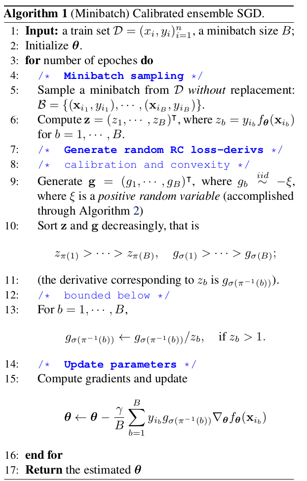
where \(\mathbf{1}(\cdot)\) is an indicator function.
Aim. To obtain the Bayes classifier or the best classifier:
$$f^* := \argmin R(f)$$
$$R(f) = 1 - \text{Acc}(f) = \mathbb{E}( \mathbf{1}(Y f(\mathbf{X}) \leq 0) ),$$
Background
Due to the discontinuity of the indicator function:
$$R(f) = 1 - \text{Acc}(f) = \mathbb{E}( \mathbf{1}(Y f(\mathbf{X}) \leq 0) ),$$
the zero-one loss is usually replaced by a convex and classification-calibrated loss \(\phi\) to facilitate the empirical computation (Lin, 2004; Zhang, 2004; Bartlett et al., 2006):
$$ R_{\phi}(f) = \mathbb{E}( \phi(Y f(\mathbf{X})) ) $$
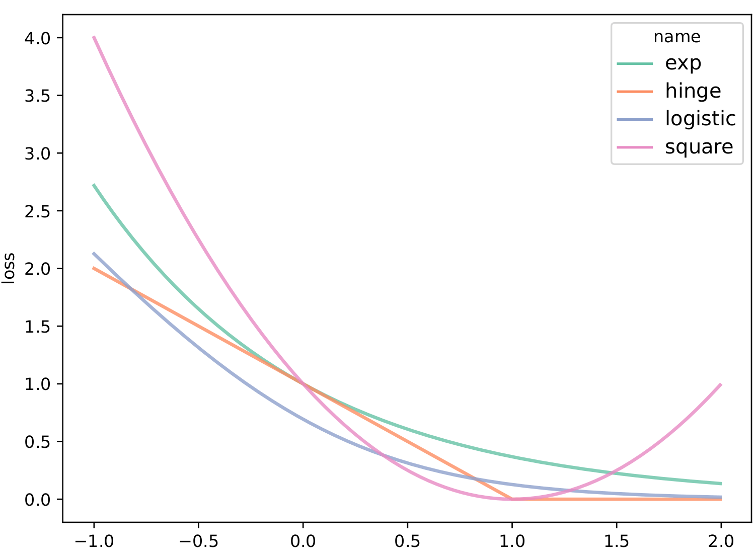
For example, the hinge loss for SVM, exponential loss for AdaBoost, and logistic loss for logistic regression all follow this framework.
Background
Due to the discontinuity of the indicator function:
$$R(f) = 1 - \text{Acc}(f) = \mathbb{E}( \mathbf{1}(Y f(\mathbf{X}) \leq 0) ),$$
(If we optimize with respect to \(\phi\), will the resulting solution still be the function \(f^*\) that we need?)
That's why we need the loss \(\phi\) to be calibrated?
$$ R_{\phi}(f) = \mathbb{E}( \phi(Y f(\mathbf{X})) ) $$
For example, the hinge loss for SVM, exponential loss for AdaBoost, and logistic loss for logistic regression all follow this framework.
the zero-one loss is usually replaced by a convex and classification-calibrated loss \(\phi\) to facilitate the empirical computation (Lin, 2004; Zhang, 2004; Bartlett et al., 2006):
Background
Definition 1 (Bartlett et al. (2006)). A loss function \(\phi(\cdot)\) is classification-calibrated, if for every sequence of measurable function \(f_n\) and every probability distribution on \( \mathcal{X} \times \{\pm 1\}\),
$$R_{\phi}(f_n) \to \inf_{f} R_{\phi}(f) \ \text{ implies that } \ R(f_n) \to \inf_{f} R(f).$$
A calibrated loss function \(\phi\) guarantees that any sequence \(f_n\) that optimizes \(R_\phi\) will eventually also optimize \(R\), thereby ensuring consistency in maximizing classification accuracy.
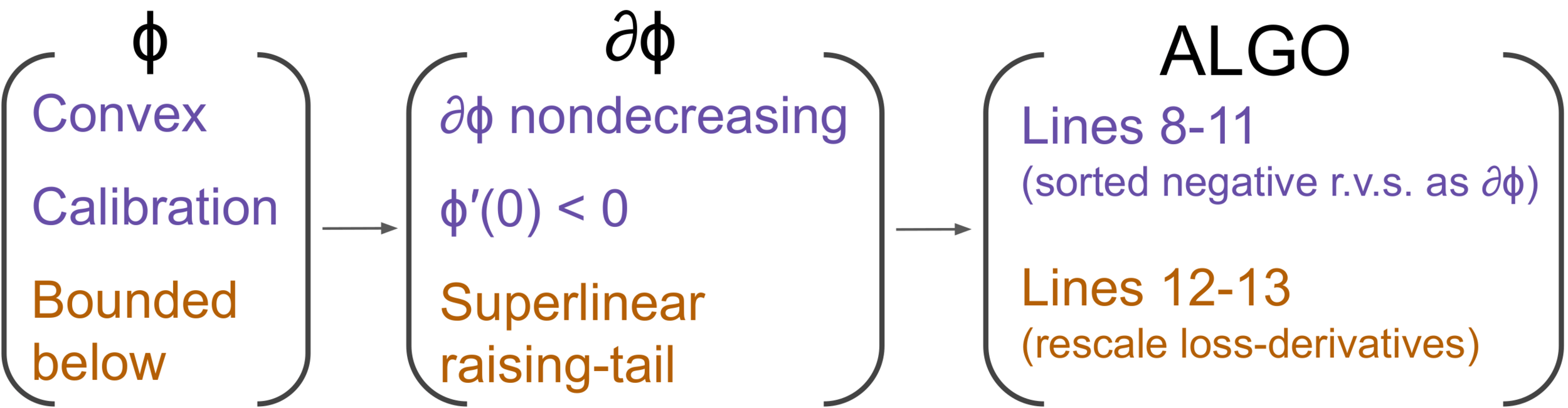
Theorem 1 (Bartlett et al. (2006)) Let \(\phi\) be convex. Then \(\phi\) is classification-calibrated iff it is differentiable at 0 and \(\phi'(0) < 0\).
A series of studies (Lin, 2004; Zhang, 2004; Bartlett et al., 2006) culminates in the following theorem for iff conditions of calibration:
Classification ERM framework
(i) Select a convex and calibrated (CC) loss function \(\phi\)
Classification ERM framework
$$ \widehat{f}_{n} = \argmin_{f \in \mathcal{F}} \ \widehat{R}_{\phi} (f), \quad \widehat{R}_{\phi} (f) := \frac{1}{n} \sum_{i=1}^n \phi \big( y_i f(\mathbf{x}_i) \big).$$
(i) Select a convex and calibrated (CC) loss function \(\phi\)
(ii) Directly minimizes the ERM of \(R_\phi\) to obtain \(f_n\)
(SGD is widely adopted for its scalability and generalization when dealing with large-scale datasets and DL models)
$$\pmb{\theta}^{(t+1)} = \pmb{\theta}^{(t)} - \gamma \frac{1}{B} \sum_{i \in \mathcal{I}_B} \nabla_{\pmb{\theta}} \phi( y_{i} f_{\pmb{\theta}^{(t)}}(\mathbf{x}_{i}) )$$
$$= \pmb{\theta}^{(t)} - \gamma \frac{1}{B} \sum_{i \in \mathcal{I}_B} \partial \phi( y_{i} f_{\pmb{\theta}^{(t)}}(\mathbf{x}_{i}) ) \nabla_{\pmb{\theta}} f_{\pmb{\theta}^{(t)}}(\mathbf{x}_{i}),$$
The ERM paradigm with calibrated losses, when combined with ML/DL models and optimized using SGD, has achieved tremendous success in numerous real-world applications.
$$\pmb{\theta}^{(t+1)} = \pmb{\theta}^{(t)} - \gamma \frac{1}{B} \sum_{i \in \mathcal{I}_B} \nabla_{\pmb{\theta}} \phi( y_{i} f_{\pmb{\theta}^{(t)}}(\mathbf{x}_{i}) )$$
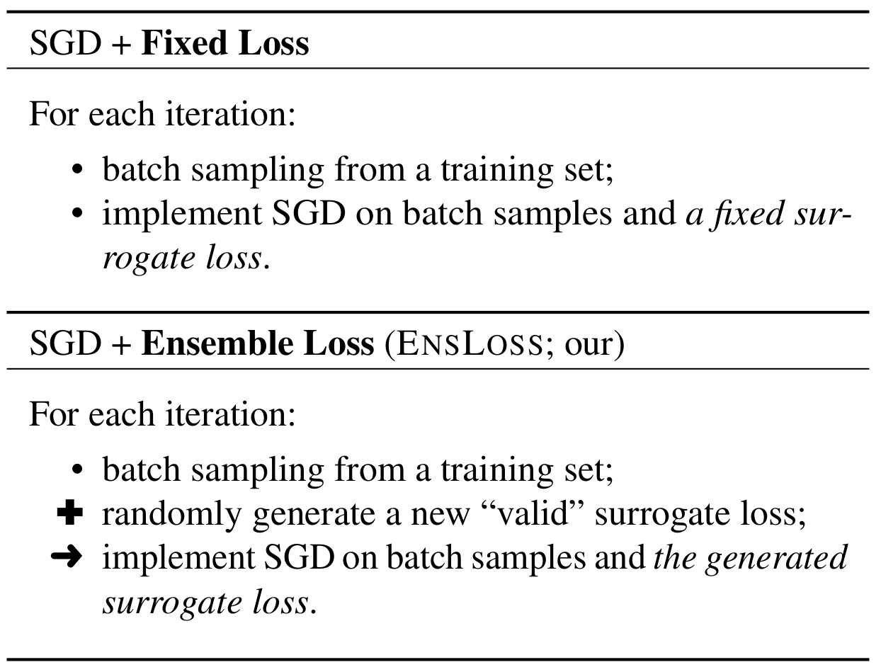
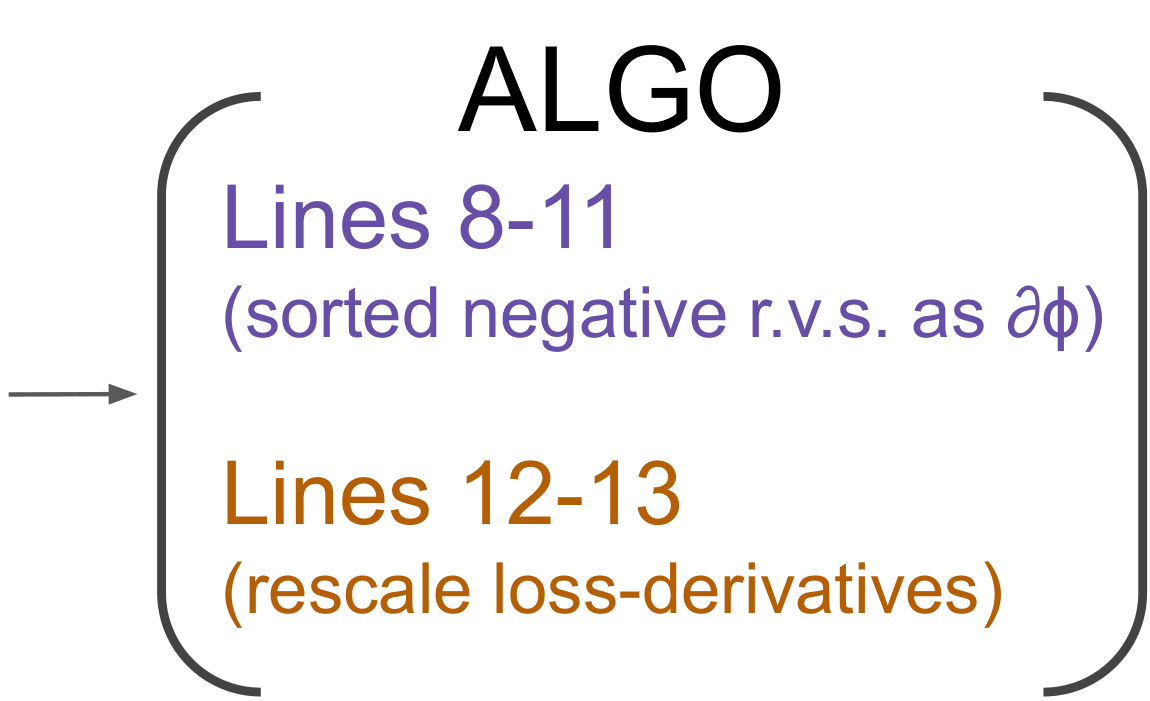
EnsLoss: Calibrated Loss Ensembles
Inspired by Dropout
(model ensemble over one training process)
$$\pmb{\theta}^{(t+1)} = \pmb{\theta}^{(t)} - \gamma \frac{1}{B} \sum_{i \in \mathcal{I}_B} \nabla_{\pmb{\theta}} \phi( y_{i} f_{\pmb{\theta}^{(t)}}(\mathbf{x}_{i}) )$$
EnsLoss: Calibrated Loss Ensembles
Inspired by Dropout
(model ensemble over one training process)
$$= \pmb{\theta}^{(t)} - \gamma \frac{1}{B} \sum_{i \in \mathcal{I}_B} \partial \phi( y_{i} f_{\pmb{\theta}^{(t)}}(\mathbf{x}_{i}) ) \nabla_{\pmb{\theta}} f_{\pmb{\theta}^{(t)}}(\mathbf{x}_{i}),$$
EnsLoss: Calibrated Loss Ensembles
$$\pmb{\theta}^{(t+1)} = \pmb{\theta}^{(t)} - \gamma \frac{1}{B} \sum_{i \in \mathcal{I}_B} \nabla_{\pmb{\theta}} \phi( y_{i} f_{\pmb{\theta}^{(t)}}(\mathbf{x}_{i}) )$$
$$= \pmb{\theta}^{(t)} - \gamma \frac{1}{B} \sum_{i \in \mathcal{I}_B} \partial \phi( y_{i} f_{\pmb{\theta}^{(t)}}(\mathbf{x}_{i}) ) \nabla_{\pmb{\theta}} f_{\pmb{\theta}^{(t)}}(\mathbf{x}_{i}),$$
EnsLoss
Experiments
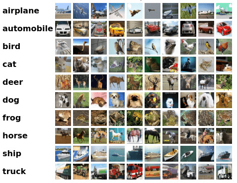
CIFAR
We construct binary CIFAR (CIFAR2), by selecting all possible pairs from CIFAR10, resulting:
10 x 9 / 2 = 45
CIFAR2 datasets.
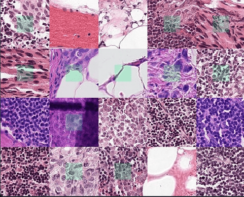
PCam
PCam is a binary image classification dataset comprising 327,680 96x96 images from histopathologic scans of lymph node sections
Experiments
OpenML
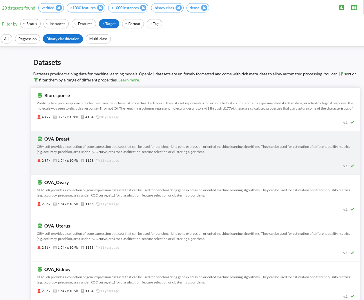
We applied a filering:
n >= 1000
d >= 1000
at least one official run
resulting 14 datasets
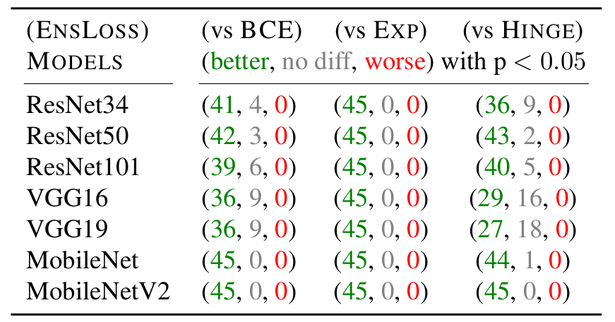
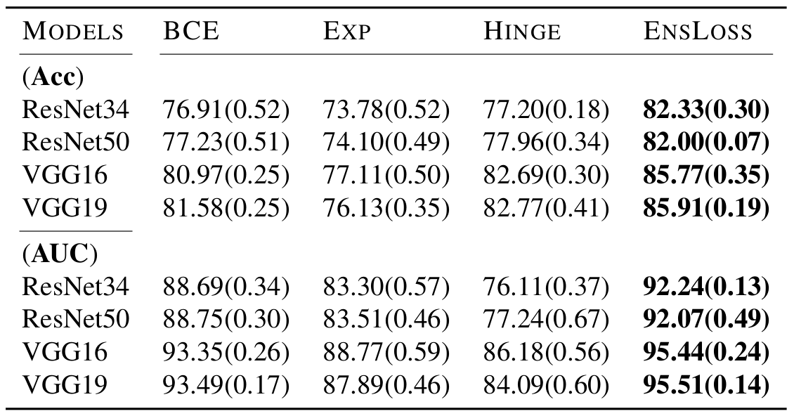
CIFAR2
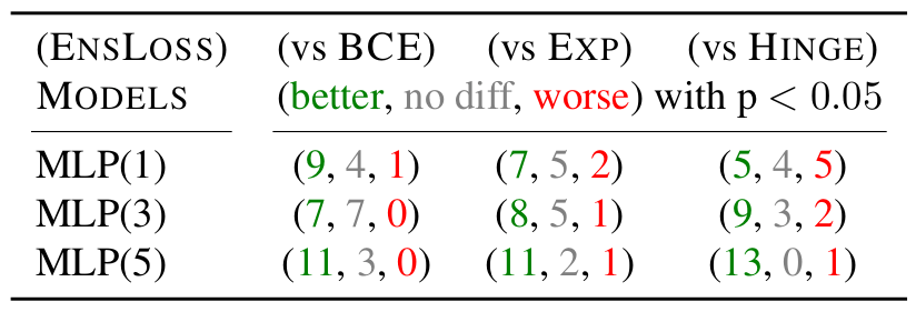
OpenML
PCam
EnsLoss is a more desirable option compared to fixed losses in image data;
and it is a viable option worth considering in tabular data.
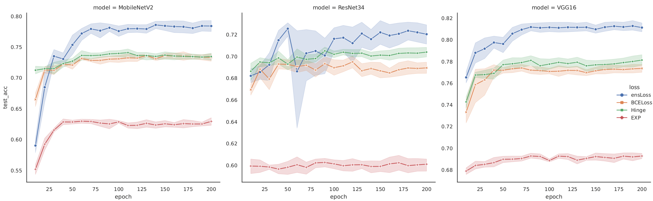
Epoch-level performance
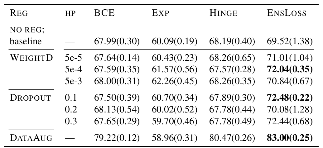
Compatibility of prevent-overfitting methods
EnsLoss consistently outperforms the fixed losses across epochs;
and it is compatible with other methods, and their combination yields additional improvement.
Summary
The primary motivation of EnsLoss behind consists of two components: “ensemble” and the “CC” of the loss functions.
This concept can be extensively applied to various ML problems, by identify the specific conditions for loss consistency or calibration.
Thank you!


ensLoss_mini
By statmlben
ensLoss_mini
[ICML2025] EnsLoss: Stochastic Calibrated Loss Ensembles for Preventing Overfitting in Classification


