Introduction to Linear Modeling
Regression Analysis
DISCLAIMER: The images, code snippets...etc presented in this presentation were collected, copied and borrowed from various internet sources, thanks & credit to the creators/owners
Agenda
-
Machine Learning
-
Regression Analysis
-
Simple Linear Regression
-
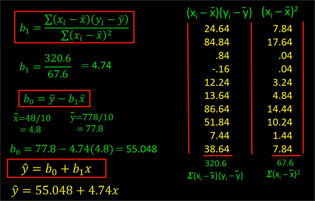
Ordinary Least Square Method
-
Example - 1
-
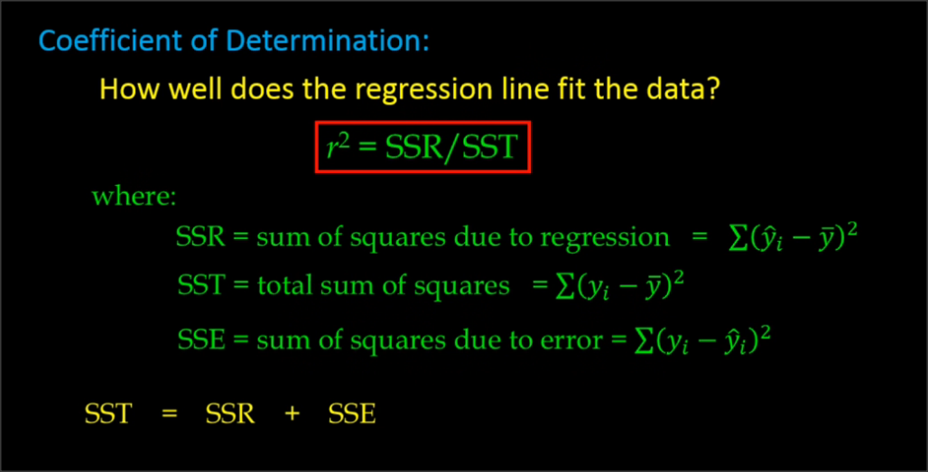
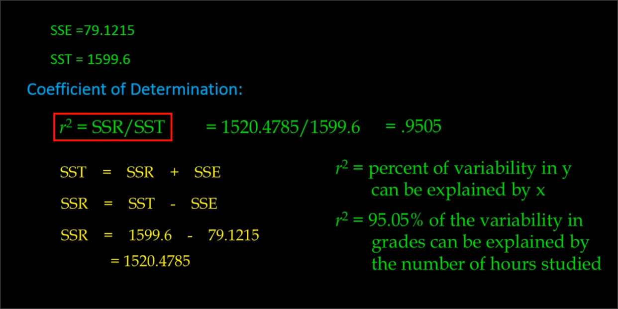
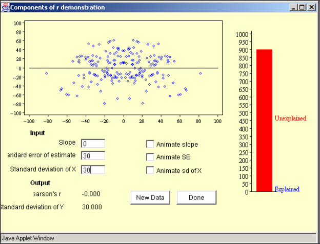
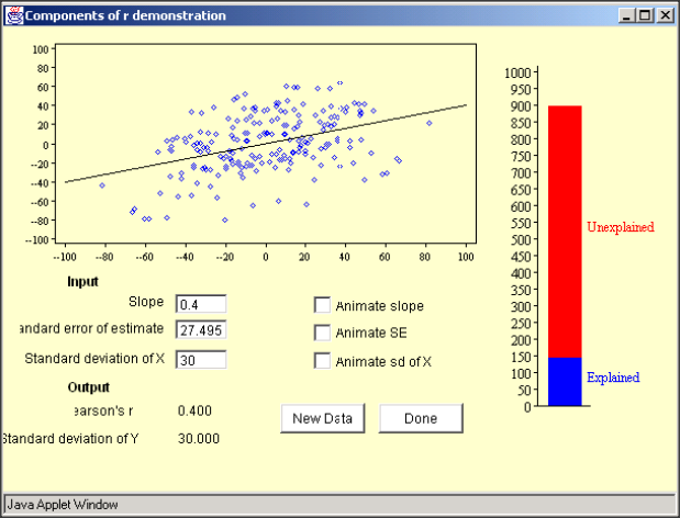
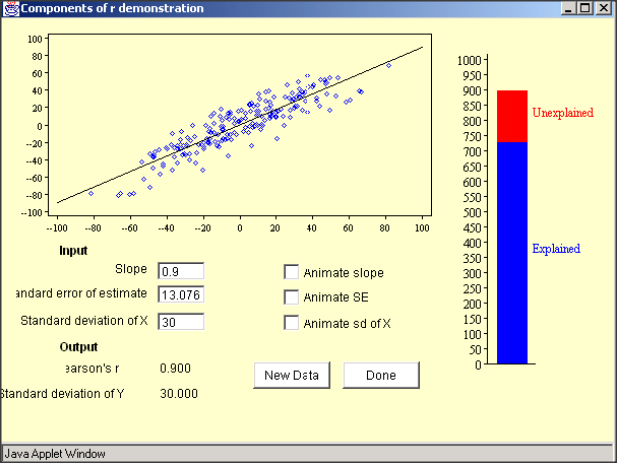
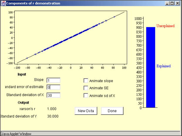
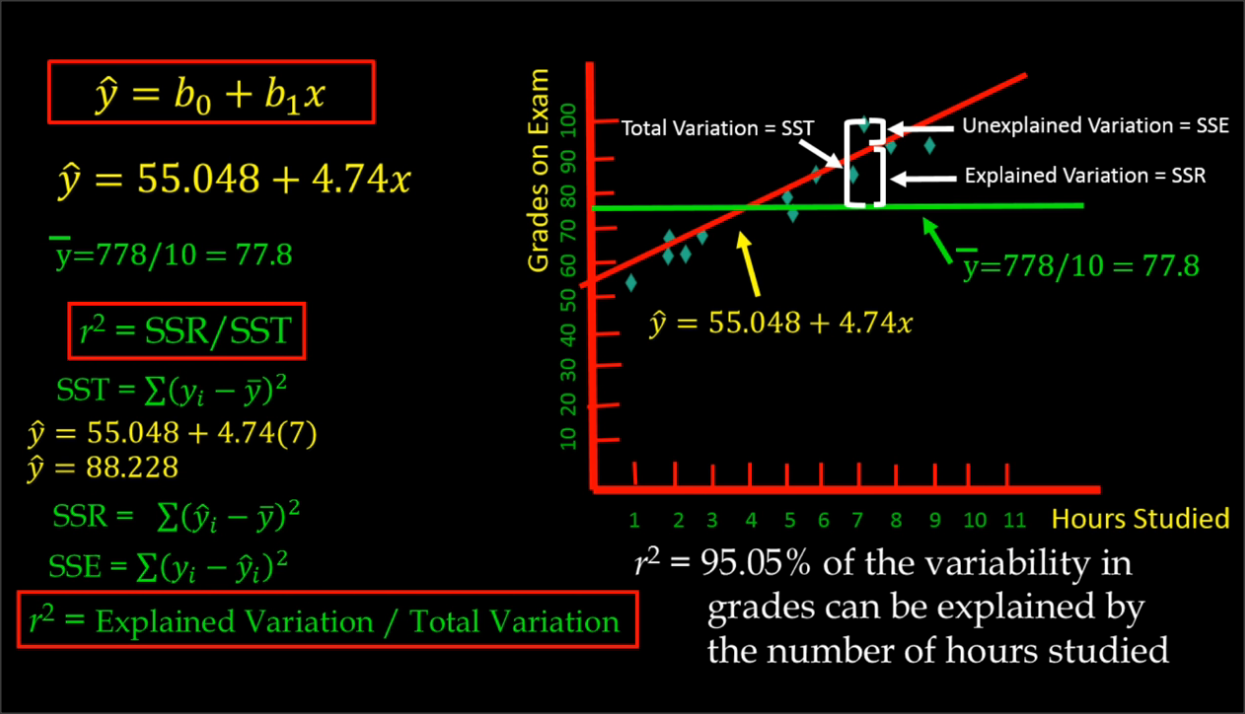
Coefficient of Determination (R-Square)
-
Example - 2
-
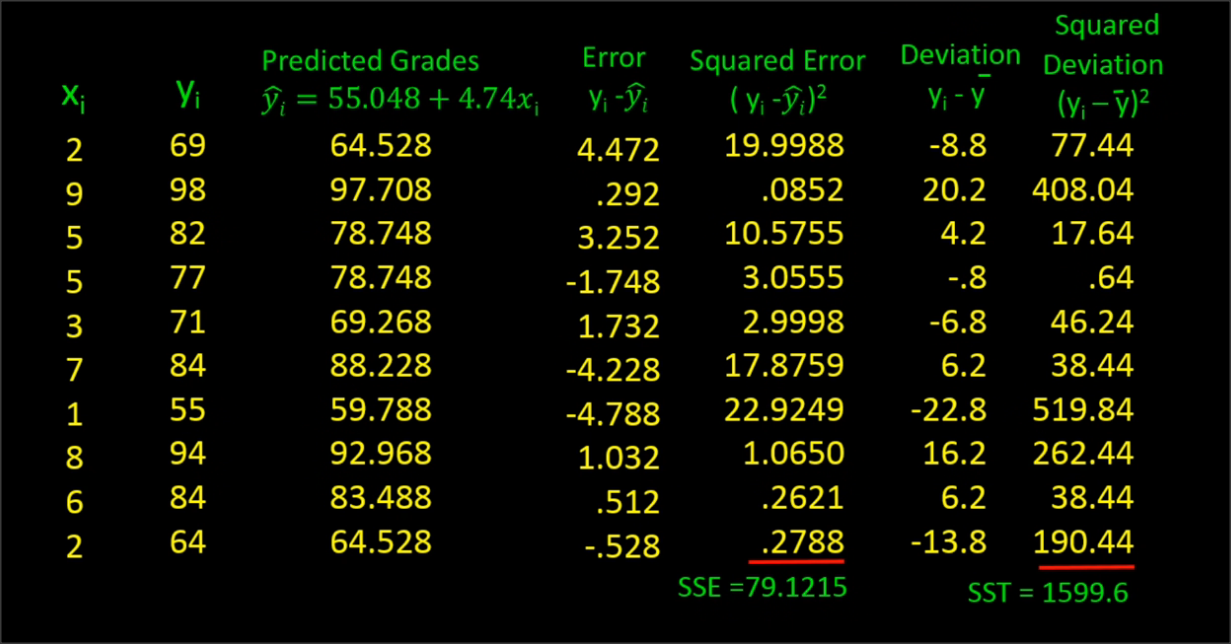
Sum of Squares Regression (SSR)
-
Total Sum of Squares (SST)
-
Sum of Square Errors (SSE)
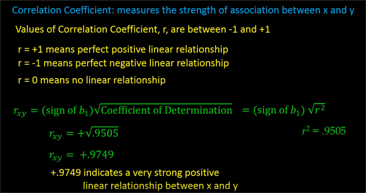
- Correlation Coefficient
Machine Learning
(what it does)
Find patterns in the data
Use those patterns to predict
the future
Regression models are used for predicting a real value
Regression Analysis
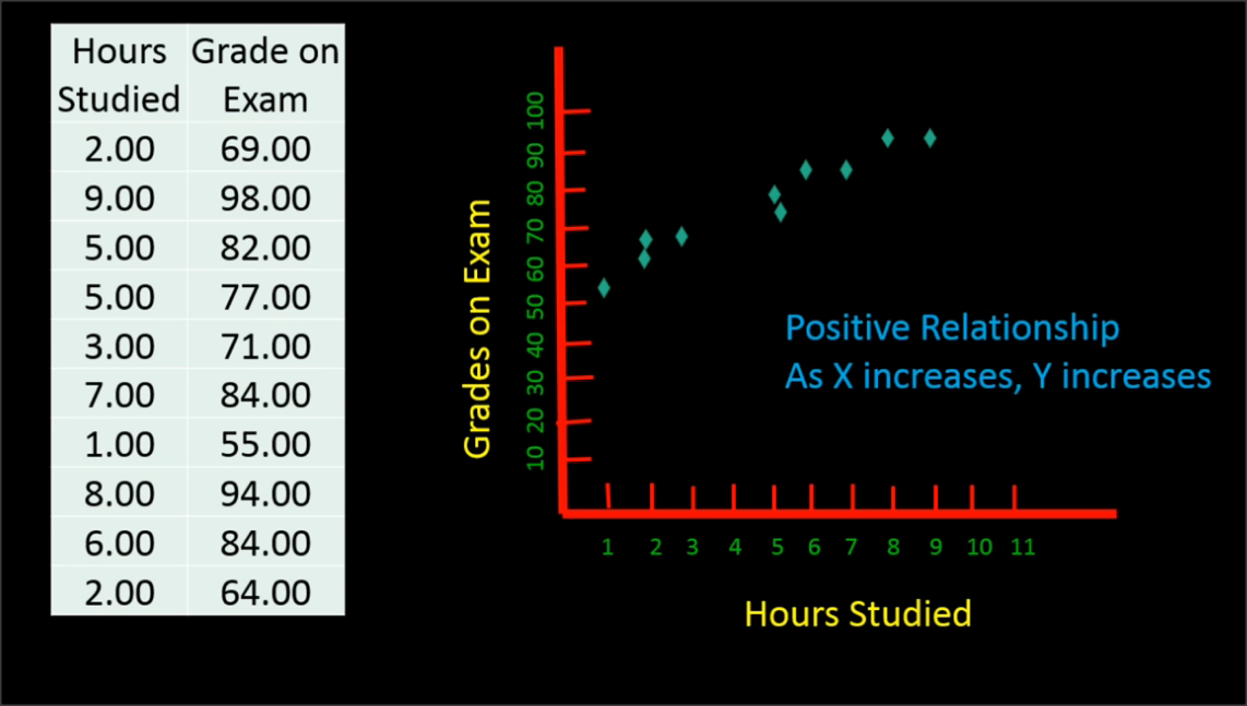
Studying the relation between two or more variables using Regression technique
Ex: relationship between advertising expenditure and sales
Simple Linear Regression


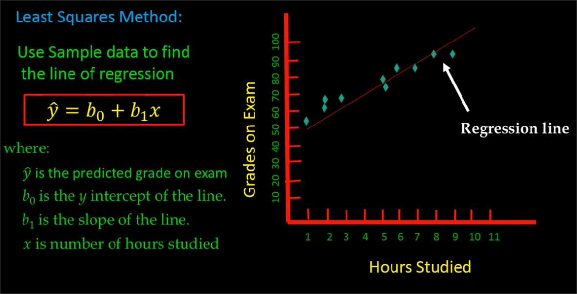
Y-intercept
or
Slope
or
error term
simple - one independent variable & one dependent variable
formula
the variable we are trying to predict
the variable we use to predict the dependent variable


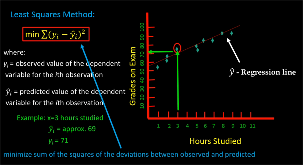
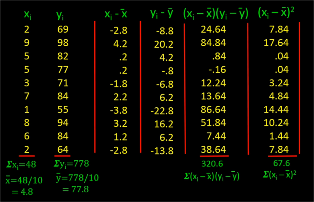
Ordinary Least Square Regression
import the data & split into training and test dataset
# Simple Linear Regression

# Importing the dataset
dataset = read.csv('Land_Price.csv')
cor(dataset$Price,dataset$Land)
# Splitting the dataset into the Training set and Test set
# install.packages('caTools')
library(caTools)
set.seed(123)
split = sample.split(dataset$Price, SplitRatio = 2/3)
training_set = subset(dataset, split == TRUE)
test_set = subset(dataset, split == FALSE)Example - 1
Fitting the model & Predicting new data
# Fitting Simple Linear Regression to the Training set
regressor = lm(formula = Price ~ Land,
               data = training_set)

# Predicting the Test set results
y_pred = predict(regressor, newdata = test_set)
Visualising the Training & Test set results
# Visualising the Training set results
library(ggplot2)
ggplot() +
  geom_point(aes(x = training_set$Land, y = training_set$Price),
             colour = 'red') +
  geom_line(aes(x = training_set$Land, y = predict(regressor, newdata = training_set)),
            colour = 'blue') +
  ggtitle('Price vs Land (Training set)') +
  xlab('Land') +
  ylab('Price')

# Visualising the Test set results
library(ggplot2)
ggplot() +
  geom_point(aes(x = test_set$Land, y = test_set$Price),
             colour = 'red') +
  geom_line(aes(x = training_set$Land, y = predict(regressor, newdata = training_set)),
            colour = 'blue') +
  ggtitle('Price vs Land (Training set)') +
  xlab('Land') +
  ylab('Price')
Example - 2
Other Sources for adv study
Other Models (SVM)
#svm
library(e1071)
# quick look at the data
plot(iris)

# feature importance
plot(iris$Sepal.Length, iris$Sepal.Width, col=iris$Species)
plot(iris$Petal.Length, iris$Petal.Width, col=iris$Species)
#split data
s <- sample(150, 100)
col <- c('Petal.Length','Petal.Width','Species')
iris_train <- iris[s,col]
iris_test <- iris[-s,col]
#create model
svmfit <- svm(Species ~ ., data = iris_train, kernel="linear", cost=.1, scale = FALSE)
print(svmfit)
plot(svmfit, iris_train[, col])

tuned <- tune(svm, Species~., data = iris_train, kernel='linear', ranges = list(cost=c(0.001, 0.01,.1, 1.10, 100)))
summary(tuned)

p <- predict(svmfit, iris_test[,col], type='class')
plot(p)
table(p, iris_test[,3])
mean(p==iris_test[,3])
Support Vector Machine (Classification)
Machine Learning - Linear Models
By sumendar karupakala
Machine Learning - Linear Models
Demonstration


