A Deep Dive into
Hyperparameter Optimization
By-
Tanay Agrawal
Data Scientist @Curl Tech
A little about me!
-
Data Scientist at Curl Tech.
-
Authored the Book; "Hyperparameter Optimization in Machine Learning".
-
Delivered talks at several conferences.
-
Write Technical Blogs.
-
Love to Read, Write, Travel and I am a Nature Enthusiast.

Let's start with the understanding what Hyperparameters are!
y = f(\theta_i, \theta_0) = \theta_i.x_i + \theta_0
Hypothesis Function for Linear Regression-
Let's understand Hyperparameters with classic example of House Pricing Dataset and Linear Regression
where, i \epsilon [1, n]
x_1
x_2
x_3
.
.
.
x_n
Number of Bedrooms
Distance from Airport
Area of House

y
House Price
etc.
We find these
\theta_s
using Optimization Algorithms
Such as Gradient Descent
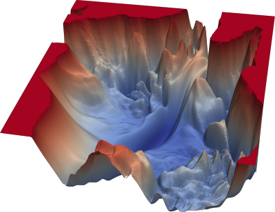
A graph of Loss Function
Learning Rate(Length of steps)
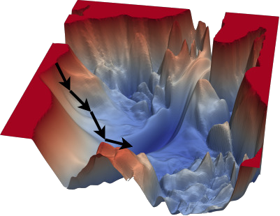
Loss function moving towards minima, while tuning weights and biases
\theta
Parameter
\alpha
Hyperparameter
Weights;
Learning rate;
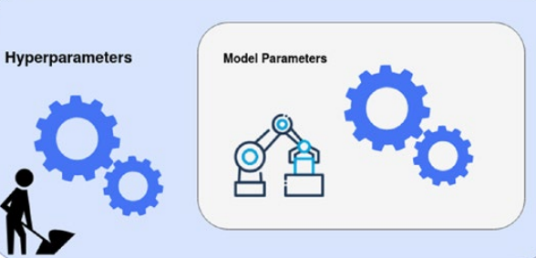
Machine Learning Model
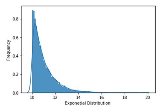
Let's now see some of the common distribution for ranges of Hyperparameters.
The distribution of the range depends on the functionality of Hyperparameter
h1 - [0.01, 0.1, 10, 100, 1000, 10000]
h2 - [2, 3, 4, 5]
h3 - [2, 4, 8, 16, 32, 64, 128, 256...]
A Hyperparameter can select values from two basic kind of distributions;
- Discrete
- Continuous
Discrete Distribution
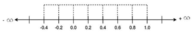
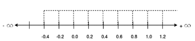
Continuous Distribution

\infty
-\infty
+\infty
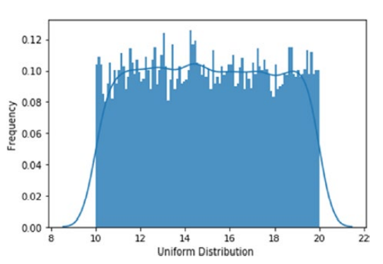
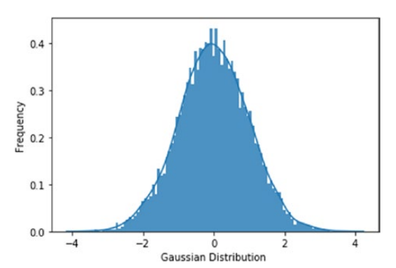
Probabilistic Distribution
Probabilistic Distribution defines the likelihood of a value the variable(here hyperparameter) can assume. Probabilistic Distribution can be classified into two types.
- Discrete Probabilistic Distribution
- Cotninuous Probabilistic Distribution
Some examples of Probabilistic Distribution
Now that you understand hyperparameters, their distribution types, and know the difference between model parameters and hyperparameters, let's move to the next section of brute force methods of Hyperparameter tuning.

Hyperparameter Tuning using Random Search and Grid Search
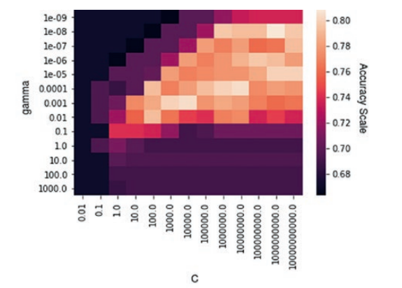
Before going to tuning, it is important to understand how change in hyperparameter can fluctuate the model performance
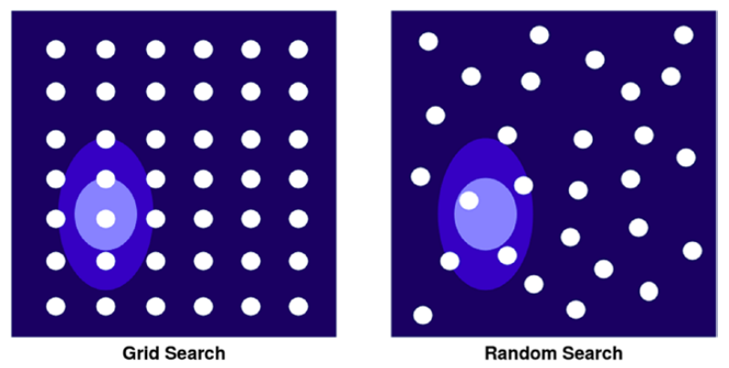
Grid Search
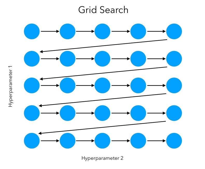
- Easy to implement.
- Cannot explore the space in Hyperparameters with Continuous ranges.
- Good option if the search space is small, and hyperparameter ranges are discrete.
- Really Slow, would be impossible to use for large search spaces, like neural networks.
Random Search
- Also easy to implement
- The number of trials fixed, hence unlike Grid Search independent of the total number of combinations.
- Non-contributing hyperparameters won't reduce the time efficiency, since a fixed number of trials.
- Can explore the continuous search space.
- Can also be used for large search spaces as it picks random combination.
- There's a possibility of leaving space which would give high accuracy.
- The number of trials needs to be decided on the basis of complexity of search space.
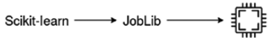
Both of these algorithms are implemented in Scikit-learn which makes them really easy to use.
Useful methods are implemented for these algorithms in scikit-learn like Cross-validation, scoring, etc.
Parallelizing Hyperparameter Optimization

Two issues while optimizing Hyperparameters
While optimizing Hyperparameters, the machine learning model is trained several times. Even when we have powerful hardware in this age, data scientists struggle two major issues:
- Time Constraint
- Memory Constrait
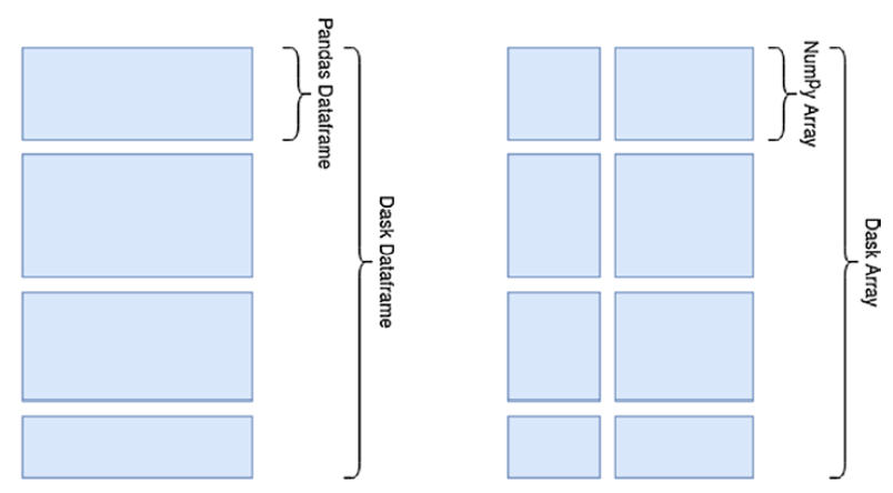
Dask
Collection
Task Graph
Multi-processing/Distribution over cluster
Collection
A dataset can be huge and might not fit into your memory. A Collection can be a dask dataframe or dask array, which consists of several smaller pandas dataframes or numpy arrays respectively. The size of chunk you can define according to your memory.
Task Graph
Task graph is the complete pipeline you want to parallelize
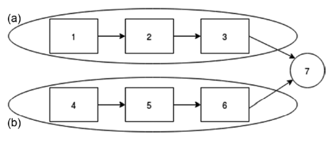
Once the task graph is done, it can be executed over a core or a cluster as per availability
dask.distributed
It's a library extended to dask for dynamic task scheduling. Client() from dask.distributed is primarily used to pass different kinds of clusters to distribute the task graph.
Example;
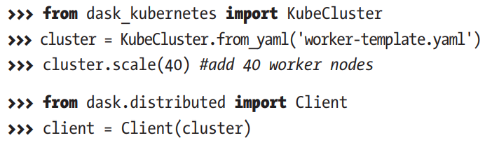
Clusters Types supported by Dask
- SSH(for unmanaged cluster)
- Kubernetes
- HPC(High-Performance Computers)
- YARN(Apache Hadoop Cluster)
- Cloud based clusters by Amazon, GCP, etc.
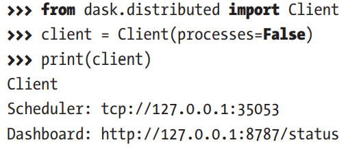
Moreover, dask provides a dashboard to track the distribution over the workers/cores, just print the client and you'll get the 'ip'.
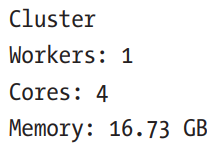
A demo of how dask can use a large dataset
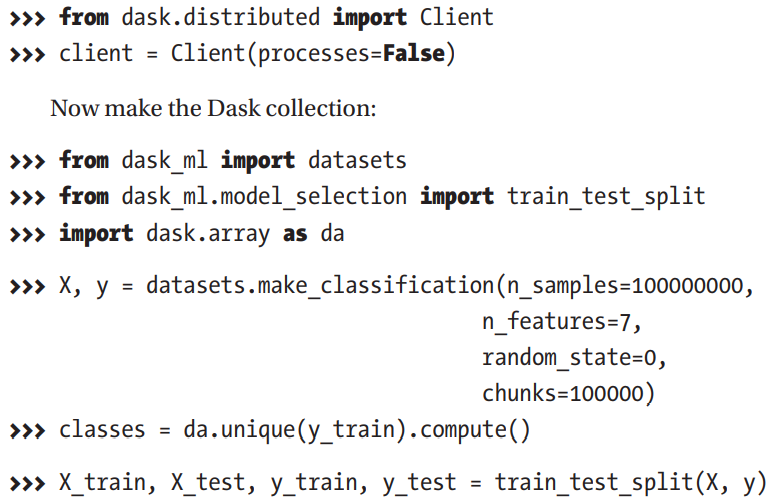
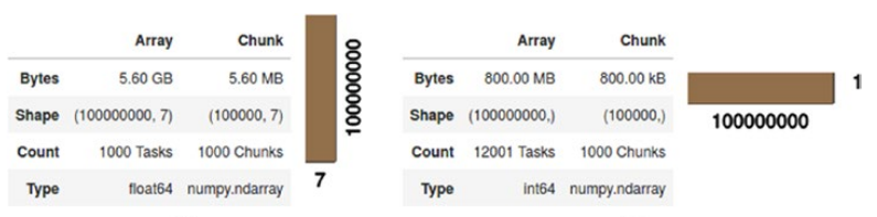
Let's train a simple model in chunks of Data using dask
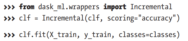

Why SGDClassifier?
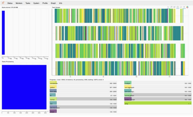
Dask Dashboard
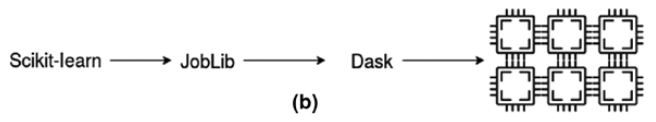
Scikit-learn with Dask
Now we'll prepare a dataset and tune hyperparameters on Scikit-learn and Scikit-learn with Dask
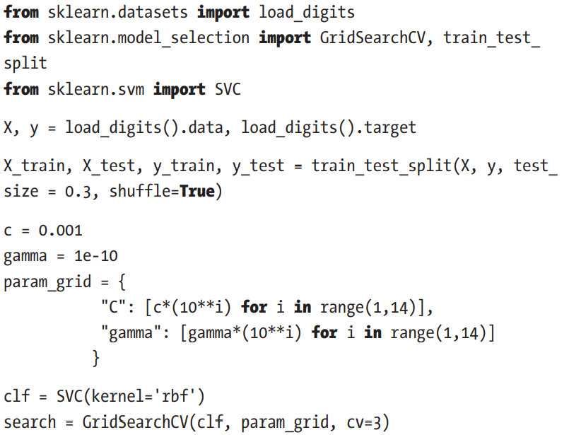
Total Size of Grid - 169
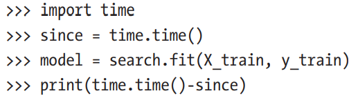
Plain and Simple Scikit-learn
Took 75.01 secs
Scikit-learn with Dask
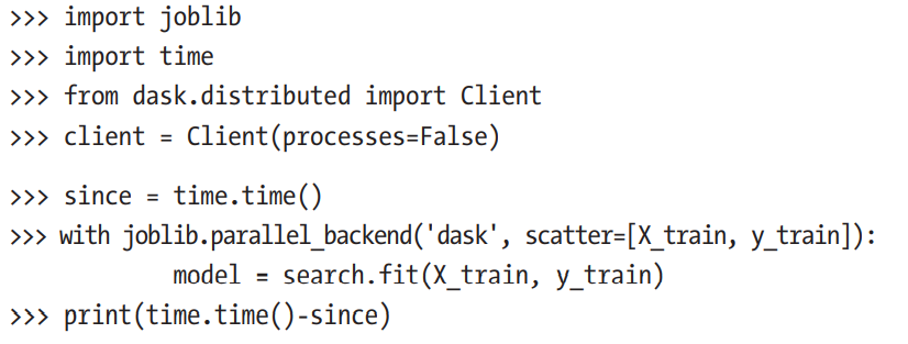
Took 34.73 secs for 169 Trials
You can use whatever cluster you want, as long the algorithm uses joblib
Note
Use scoring function while training the algorithm from dask_ml
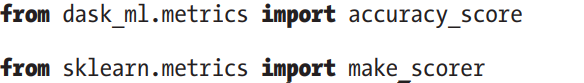

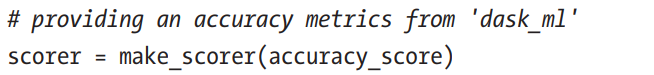
modeling algorithm uses scikit-learn's scorer by default and converts all dask array to numpy array hence filling up the memory
There are some more hyperparameter optimization algorithms in Dask
- Incremental Search
- Successive Halving
- Hyperband
Bayesian Optimization
Sequential Model-Based Global Optimization
- Uses Bayesian Optimization
- Keeps Track of previous evaluations
- Selects subsequent set of hyperparameter based on a probabilistic model
p(y|x)
Here, y is the score when our hypothesis function f is evaluated on x set of hyperparameters
How SMBO works
It has four important aspects:
- Search Space
- Objective Function
- Probabilistic Regression Model(Surrogate Function)
- Acquisition Function
Search Space(X)
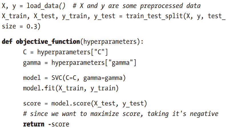
Objective Function(f)
Probabilistic Regression Model or Surrogate Model(M)
- Probabilistic Modeling of the Objective function
- Each iteration updates the surrogate function after each trial.
- Surrogate function is less costly to evaluate, it is given to acquisition function to find the next set of hyperparameters.
- Some surrogates are, TPE, GP, Random Forest, etc.
- GP Directly models p(y|x)
- TPE models p(y|x) on both p(x|y) and p(y) using conditional probability
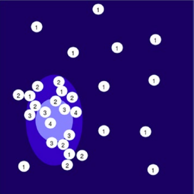
Acquisition Function(S)
The acquisition function calculates the score using the surrogate model and predicted loss on the previous set of hyperparameters. The function is then minimized or maximized depending upon the kind of acquisition function.
Usually we use EI(Expected Improvement) as Acquisition function.
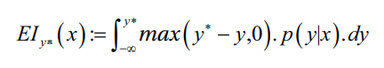
y^*
is some threshold, y=f(x) is score we get by evaluating f on set of hyperparameters x.
A positive value of the integral means there are good chances that hyperparameters proposed would yield a good score.
Summarization of SMBO steps
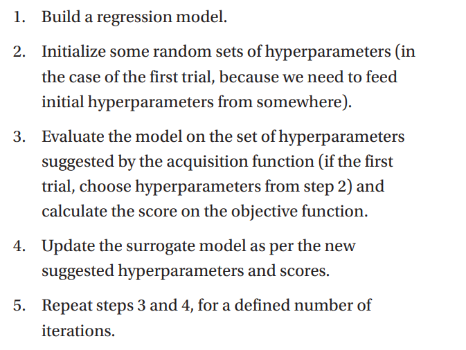
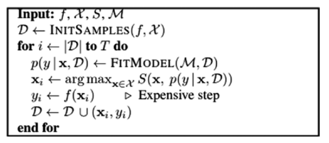
Pseudo Code
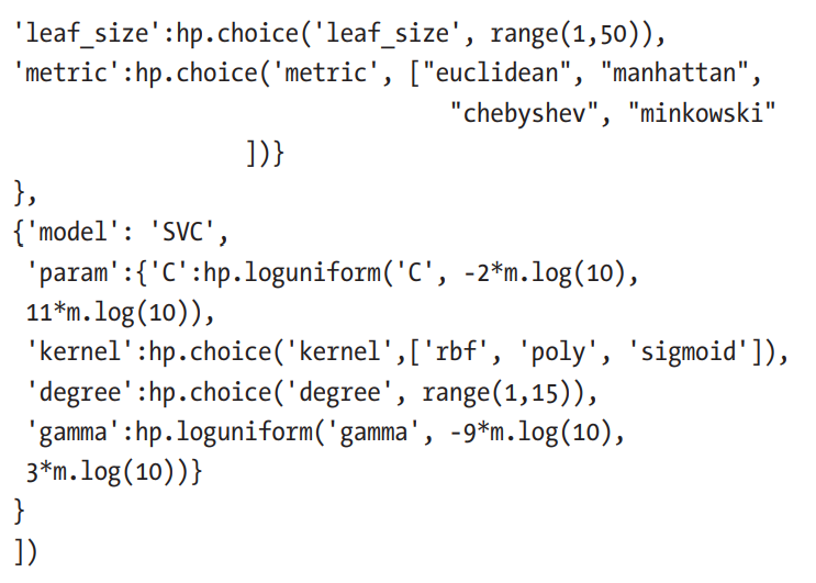
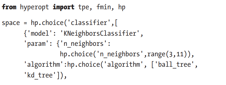
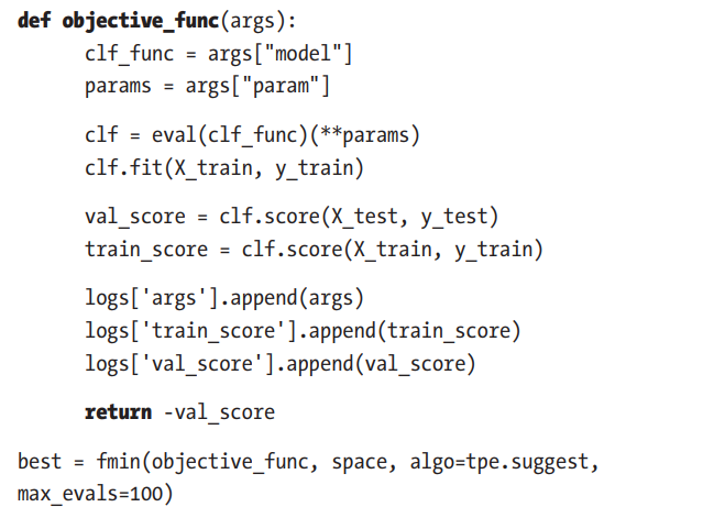
Hyperopt
Hyperopt implements, SMBO methods, it uses TPE to form Surrogate Model and Expected Improvement for Acquisition Function.
We need to provide it with two things, an Objective function and the Search Space
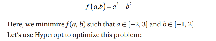
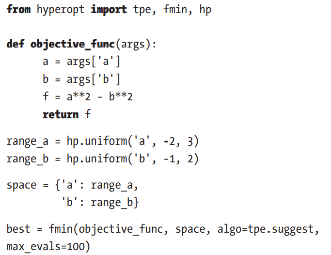
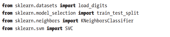
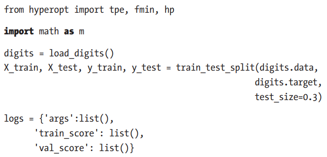
Now let's optimize a real machine learning problem
Let's now jump over to Github repo to look at some more code

If you want to dig deeper into the field, buy this awesome book :D

A Dive into Hyperparameter Optimization
By Tanay Agrawal


