Graphs of Geodesically-Convex Sets
Loose Ends, and SO(3) without SDPs
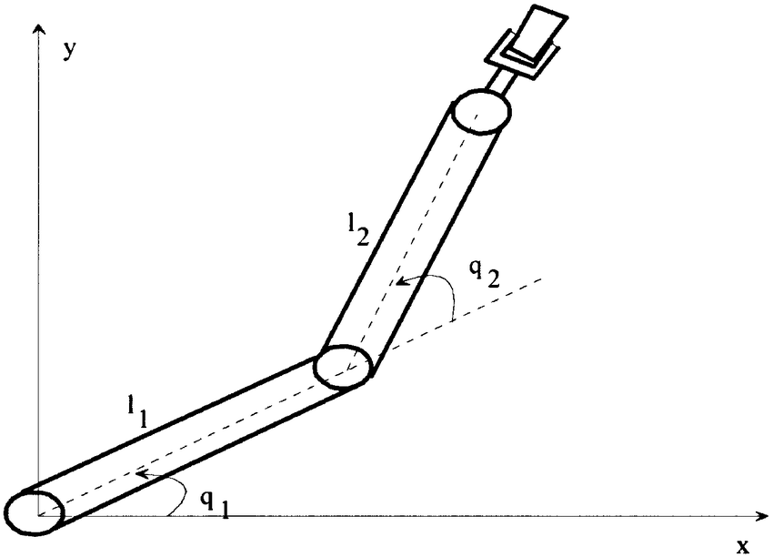
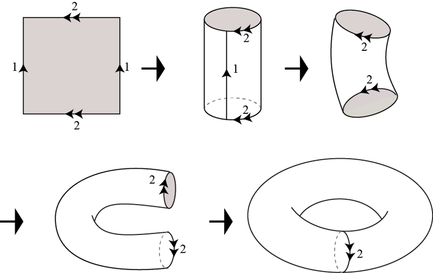
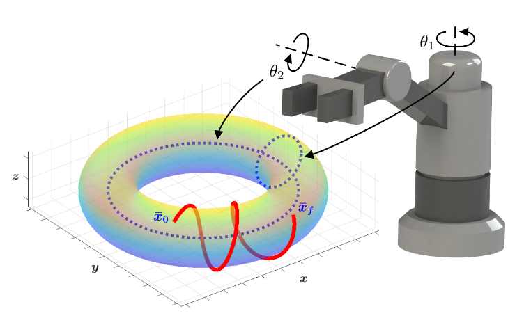
Robot Configuration Spaces as Smooth Manifolds
Robust Combined Adaptive and Variable Structure Adaptive Control of Robot Manipulators, Yu
\mathcal{Q}=\{(q_1,q_2)\,|\,0\le q_1\le 2\pi, 0\le q_2\le 2\pi\}
(No joint limits)
Survey of Graph Embeddings into Compact Surfaces, Potoczak
Trajectory Optimization on Manifolds: A Theoretically-Guaranteed Embedded Sequential Convex Programming Approach, Bonalli et. al.
Geodesics: Shortest Paths
For a curve \(\gamma\) connecting two points \(p=\gamma(0),q=\gamma(1)\) on a manifold, its arc length is
\[\int_0^1||\dot\gamma(t)||\,\mathrm{d}t\]
Geodesics on Surfaces by Variational Calculus, Villanueva
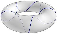
The Curvature and Geodesics of the Torus, Irons
This yields a distance metric
\[d(p,q)=\inf\{L(\gamma)\,|\,\gamma\in\mathcal{C}^{1}_{\operatorname{pw}}([0,1],\mathcal{M}),\\\gamma(0)=p,\gamma(1)=q\}\]
A geodesic is a (locally) length-minimizing curve.
Convex Sets
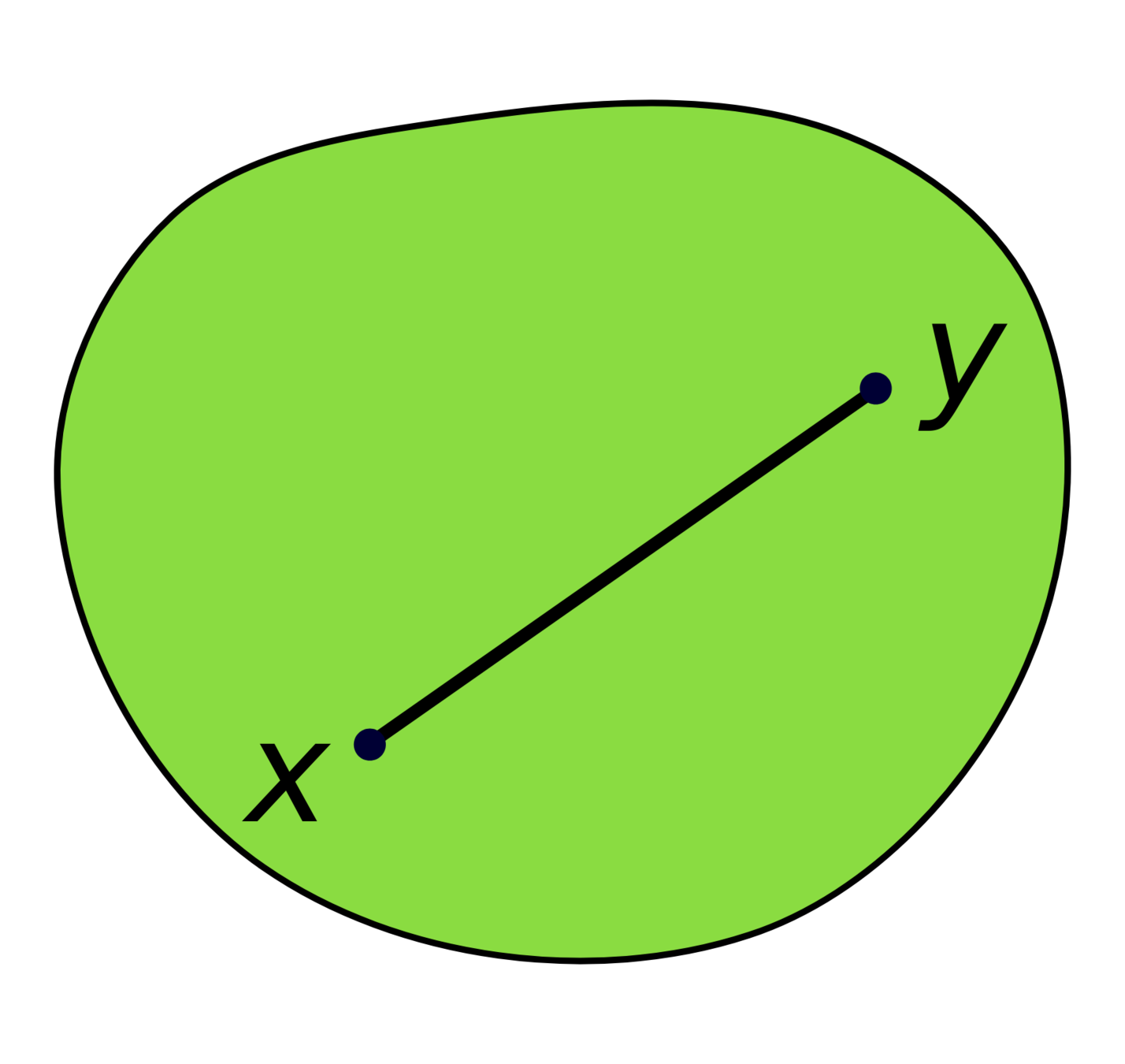
A set \(X\subseteq\mathbb{R}^n\) is convex if \(\forall p,q\in X\), the line connecting \(p\) and \(q\) is contained in \(X\)
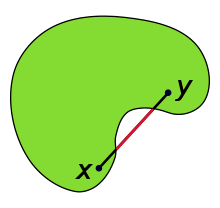
Geodesically Convex Sets
A set \(X\subseteq\mathcal{M}\) is strongly geodesically convex if \(\forall p,q\in X\), there is a unique length-minimizing geodesic (w.r.t. \(\mathcal{M}\)) connecting \(p\) and \(q\), which is completely contained in \(X\).
Convex Set, Wikipedia
Convex Functions
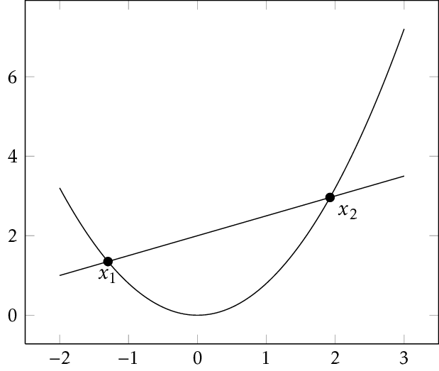
A function \(f:X\to\mathbb{R}\) is convex if for any \(x,y\in X\) and \(\lambda\in[0,1]\), we have
\[f(\lambda x+(1-\lambda)y)\le\]
\[\lambda f(x)+(1-\lambda) f(y)\]
Geodesically Convex Functions
A function \(f:\mathcal{M}\to\mathbb{R}\) is geodesically convex if for any \(x,y\in \mathcal{M}\) and any geodesic \(\gamma:[0,1]\to\mathcal{M}\) such that \(\gamma(0)=x\) and \(\gamma(1)=y\), \(f\circ\gamma\) is convex
Convex Functions
Geodesically Convex Functions
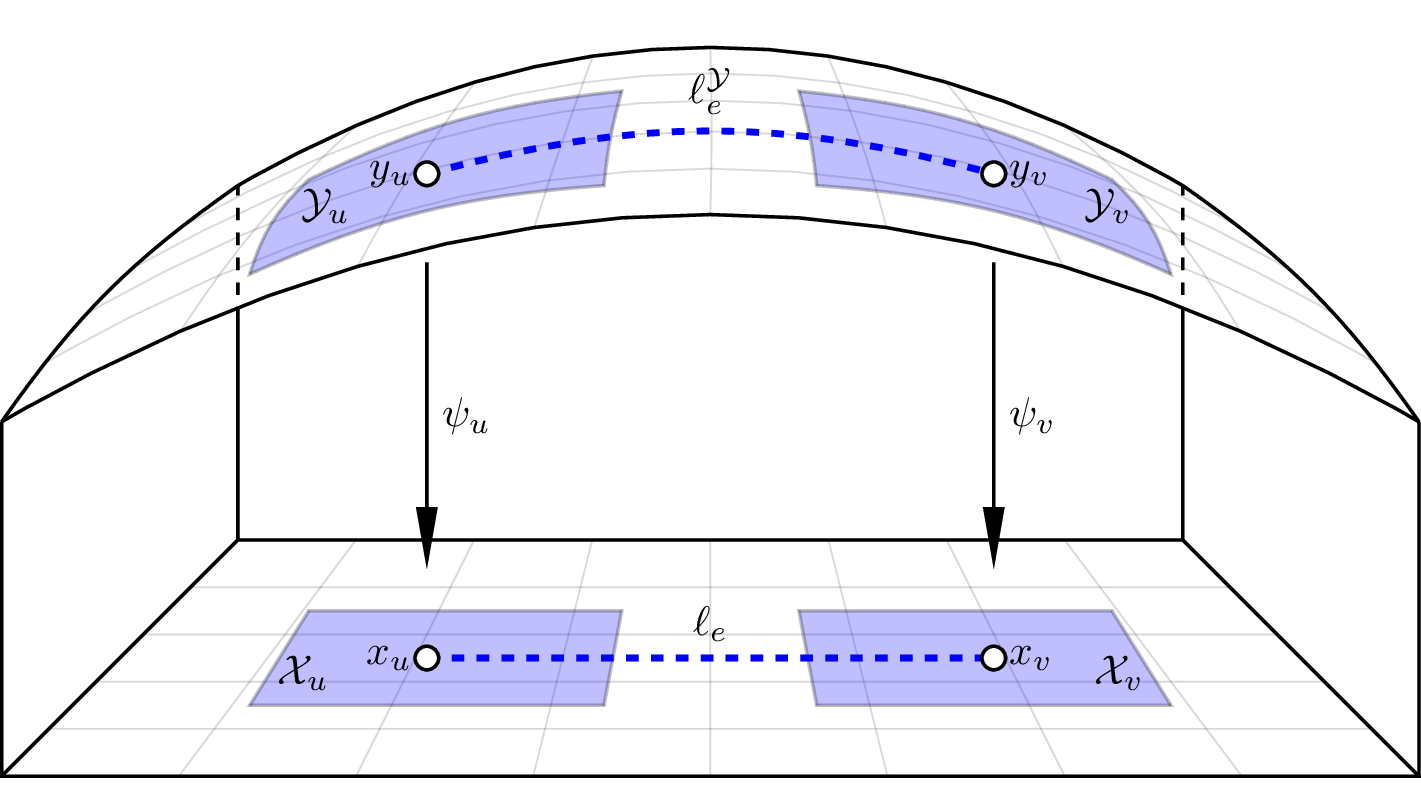
A Graph of Geodesically Convex Sets (GGCS)
A directed graph \(G=(V,E)\)
- For each vertex \(v\in V\), there is a strongly geodesically convex manifold \(\mathcal{Y}_v\)
- For each edge \(e=(u,v)\in E\), there is a cost function \(\ell_e^\mathcal{Y}:\mathcal{Y}_u\times\mathcal{Y}_v\to\mathbb{R}\)
- \(\ell_e^\mathcal{Y}\) must be geodesically convex on \(\mathcal{Y}_u\times\mathcal{Y}_v\)
Transforming Back to a GCS
When is it Convex?
Have to consider the curvature of the manifold.

Positive curvature
E.g. \(S^n,\operatorname{SO}(3),\operatorname{SE}(3)\)
Negative curvature
E.g. Saddle, PSD Cone \(\vphantom{S^n}\)
Zero curvature
E.g. \(\mathbb R^n, \mathbb T^n\)
Zero-Curvature is Still Useful
- All 1-dimensional manifolds
- Continuous revolute joints
- \(\operatorname{SO}(2)\), \(\operatorname{SE}(2)\)
- Products of flat manifolds
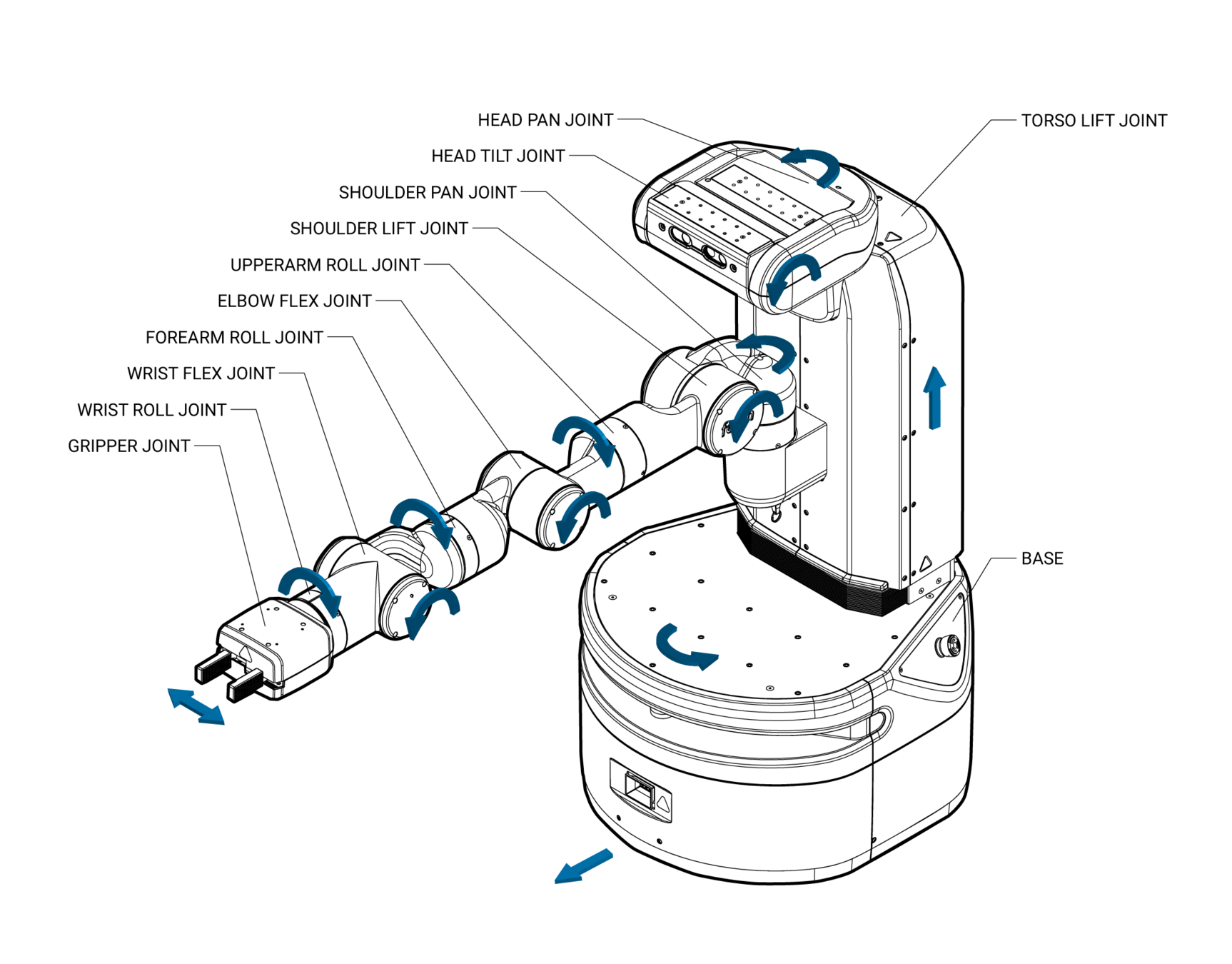
Fetch Robot Configuration
Space: \(\operatorname{SE}(2)\times \mathbb{T}^3\times \mathbb{R}^7\)
Why is Positive Curvature Bad?

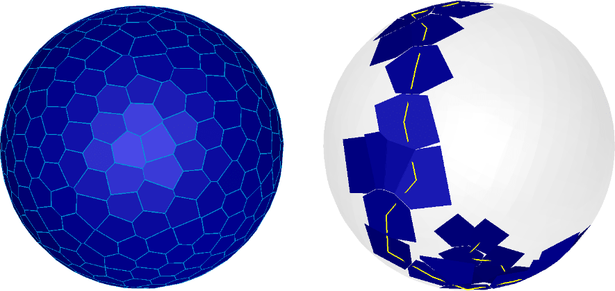
Planning on PL Approximations
Path Planning on Manifolds using Randomized Higher-Dimensional Continuation, Porta and Jaillet
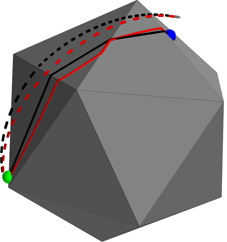
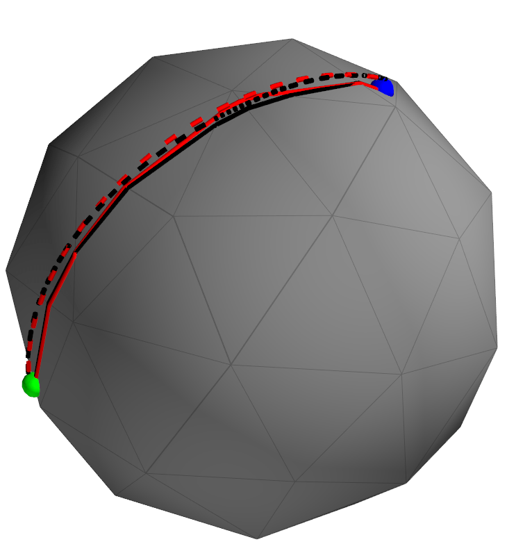
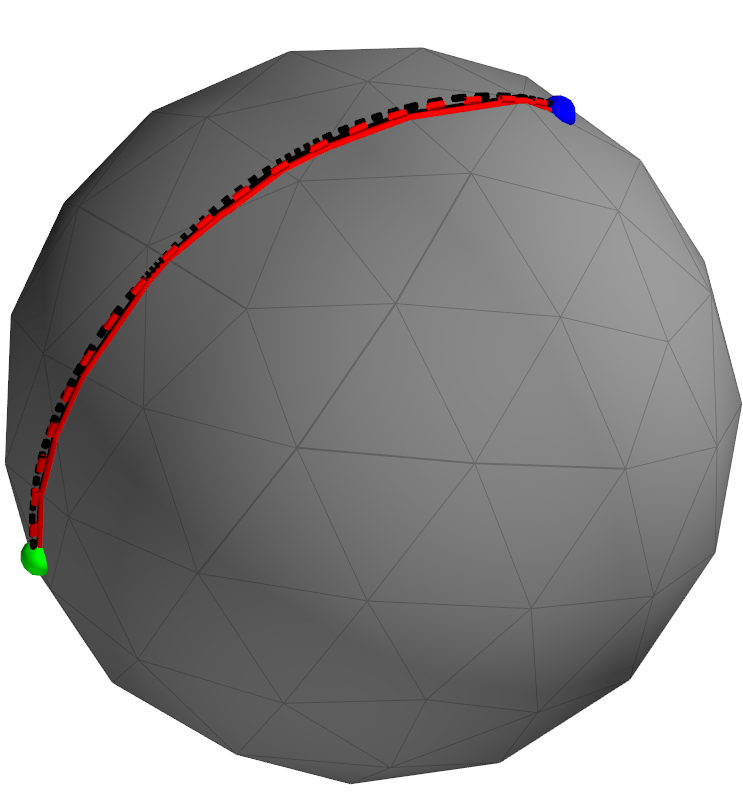
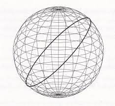
Planning on PL Approximations
Black: Shortest path on PL approximation
Red: Shortest path on sphere
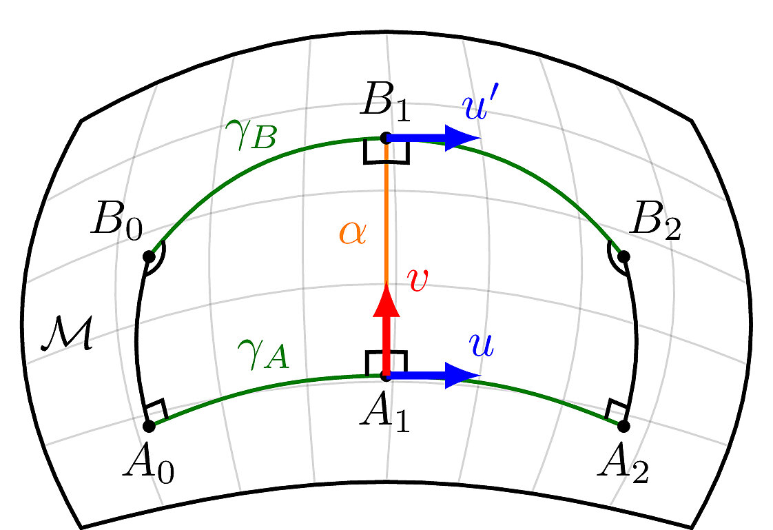
Rough Bounds on Approximation Error
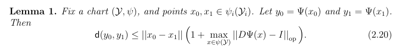
Intuition: How much does the Jacobian of the chart vary?
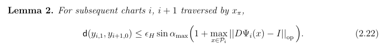
Intuition: The amount we can "slip" along the boundary also depends on the Hausdorff distance \(\epsilon_H\) between the manifold and its triangulation, as well as the angle \(\alpha_{\operatorname{max}}\) between adjacent charts.
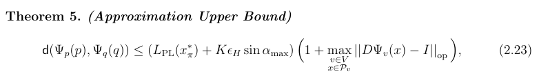
Intuition: The error grows additively with the number of sets traversed in the optimal path.
Focusing on SO(3)/SE(3)
Recall that \(\operatorname{SE}(3)\) is just \(\operatorname{SO}(3)\times\mathbb R^3\)
Three representations for \(\operatorname{SO}(3)\):
- Euler angles (\(S^1\times S^1\times S^1\))
- 27 sets, 702 edges (fully connected)
- Axis-angle (\(S^2\times S^1\))
- 60 sets, 660 edges
- Quaternions (\(S^3\))
- 27 sets and 390 edges or 64 sets and 2240 edges
\(S^1\) is flat (no approximation needed)
Numerical Comparison
Randomly sample \(n\) start and goal pairs, plan between them with each approximation.
Compute the true distance, and explore the error distribution.
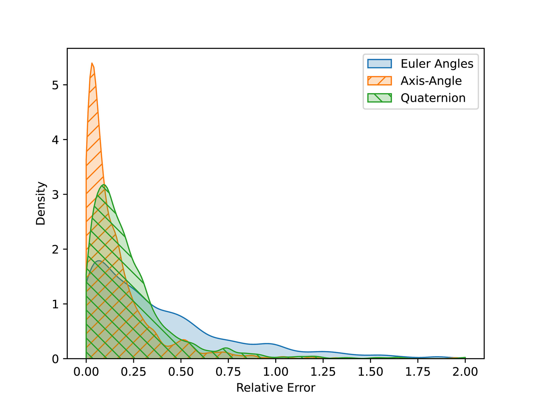
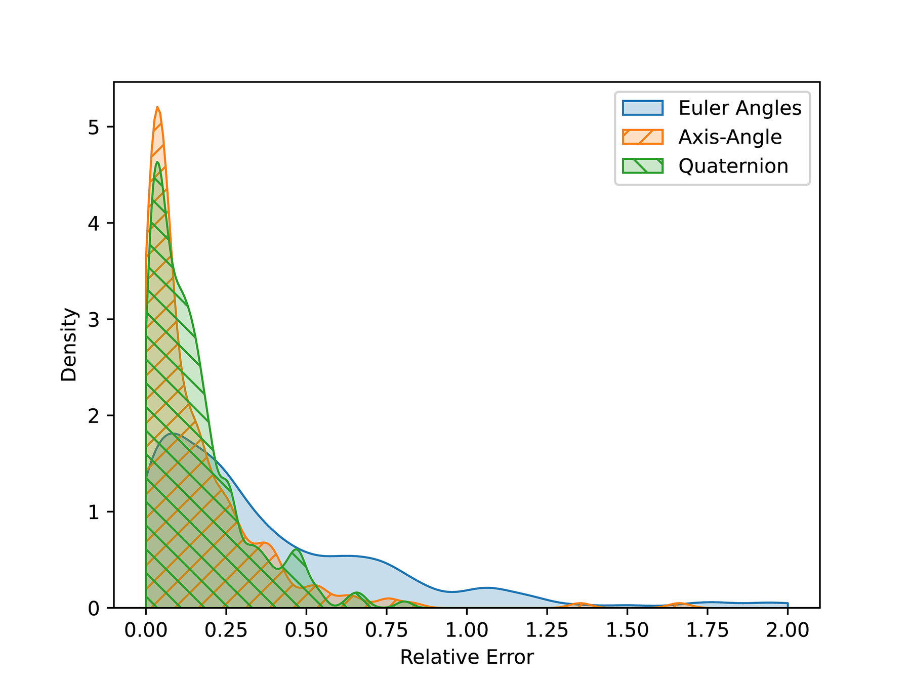
Note: two possible representations in axis-angle and quaternion, so we plan twice. Euler angles are stranger, so we ignore.
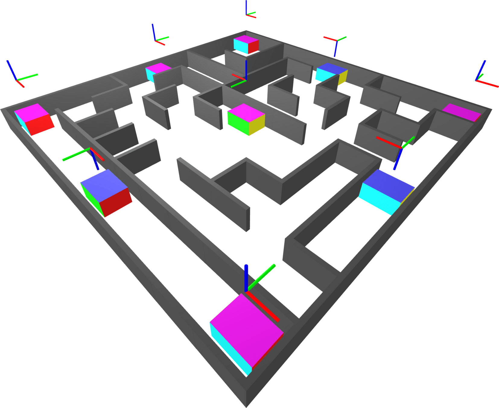
SE(3) Maze
Consider a block moving freely in 3D through a 2D maze.
Generate collision free regions with IRIS-NP. (Have to use Euler angles.)
More Setup Details
Making the graph:
- Create a grid-like roadmap
- Cover subset of edges with IRIS regions to connect key poses
200 sets, 4744 edges
- Good engineering
- Loose tolerance for relaxation (\(\sim 10^3\))
- Use L1-norm for convex relaxation (still use L2-norm for the convex restriction)
Tricks to deal with the bigger graph:
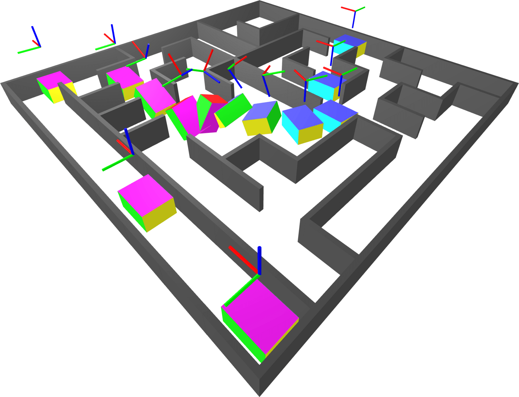
Shortest Paths in the Maze
Sample path between a start/goal pair.
The large gap in the center gives room for the block to reorient itself.
Statistics across All Pairs
GCS average runtime: 354.98 seconds
GCS* average runtime: 46.71 seconds
GCS* is ~7 times faster, and produces paths that are only 4.4% longer than GCS on average.
Takeaway: For large collision-free kinematic motion planning problems, use GCS*
What's Next?
- Shruti's talk
- SO(3) representations are non-unique, but maybe we can get around that with auxiliary vertices and edges.
- Can interpret this as a configuration-space symmetry
- I'll be talking more about this next week
RLG Group Meeting Short Talk 11/15/24
By tcohn


