Non-Euclidean Motion Planning with Graphs of Geodesically-Convex Sets


Robot Locomotion Group
Thomas Cohn, Mark Petersen, Max Simchowitz, Russ Tedrake
RQE Presentation - February 12, 2025
Outline
-
Motivation
- Robot Motion Planning
-
Context
- Mixed-Integer Optimization
- Optimization on Manifolds
-
Our Contributions
- Methodology
- Experimental Results
- Beyond Flat Manifolds
- What Comes Next?
Part 1
Motivation
Motion Planning

https://mapsplatform.google.com/maps-products/routes/
Broadly speaking
- How can I get from Point A to Point B?
- Objectives?
- Distance
- Time
- Gas
- Constraints?
- Road closures
- Avoid tolls
- Avoid ferries
Robot Motion Planning
What has changed?
- No more roads to follow
- We can move freely
- Have to avoid obstacles
- More complex motions
- Not just worrying about position in 2D
- Robot arms move in strange ways

Configuration-Space Planning
https://github.com/ethz-asl/amr_visualisations
Task Space
Configuration Space
Planning with Roadmaps
Michigan Robotics 320, Lecture 15


Standard algorithms include PRM (Kavraki 1996), PRM* (Karaman 2011), and SPARS (Dobson 2012).
Planning with Roadmaps
Pathfinding with Rapidly-Exploring Random Tree, Knox
Tree-based roadmap generators include RRT (LaValle 1998), EST (Hsu 1999), STRIDE (Gipson 2013), and FMT (Janson 2015).
Trajectory Optimization
Underactuated Robotics, Russ Tedrake

Control points of a trajectory are decision variables.
Use costs and constraints to enforce objectives, dynamics, and more.
Trajectory optimization approaches include STOMP (Kalakrishnan 2011), CHOMP (Zucker 2013), KOMO (Toussaint 2014), ALTRO (Howell 2019), cuRobo (Sundaralingam 2023).
Motion Planning Today
- Sampling-based planning
-
+
Global (probabilistic) completeness -
-
"Curse of Dimensionality" -
-
Non-smooth paths
-
- Trajectory optimization
-
-
Nonconvex -
+
Scales with dimension -
+
Smooth paths, dynamics
-
Motion Planning, Wikipedia


Motion Planning Today
- Sampling-based planning
-
+
Global(probabilistic)completeness -
-
"Curse of Dimensionality" -
-
Non-smooth paths
-
- Trajectory optimization
-
-
Nonconvex -
+
Scales with dimension -
+
Smooth paths, dynamics
-
Motion Planning, Wikipedia
- Sampling-based planning
-
+
Global (probabilistic) completeness -
-
"Curse of Dimensionality" -
-
Non-smooth paths
-
- Trajectory optimization
-
-
Nonconvex -
+
Scales with dimension -
+
Smooth paths, dynamics
-
Part 2
Context
Nonconvexity in TrajOpt

Reproduced from Slides for the Technion Robotics Seminar, Russ Tedrake
Planning through Convex Sets
Motion Planning around Convex Obstacles with Convex Optimization, Marcucci et. al.
- Want a path from \(q_0\) to \(q_T\)
- Red region: obstacle
- Blue regions (\(\mathcal Q_i\)): safe sets
Convex obstacle avoidance guarantees!
- Piecewise-linear trajectories: just check endpoints
- Bezier curves: check control points


How Do We Get Convex Sets?
Existing approaches include
- Sampling-Based Neighborhood Graph Ellipsoids (SNG)
- The Sampling-Based Neighborhood Graph: An Approach to Computing and Executing Feedback Motion Strategies (Yang and LaValle)
- Iterative Regional Inflation by Semidefinite programming (IRIS)
- Computing Large Convex Regions of Obstacle-Free Space through Semidefinite Programming (Deits and Tedrake)
- Iterative Regional Inflation by Semidefinite & Nonlinear Programming (IRIS-NP)
- Growing Convex Collision-Free Regions in Configuration Space using Nonlinear Programming (Petersen and Tedrake)
A Graph of Convex Sets
A directed graph \(G=(V,E)\)
- For each vertex \(v\in V\), there is a convex set \(\mathcal{X}_v\)
- For each edge \(e=(u,v)\in E\), there is a convex cost function \[\ell_e:\mathcal{X}_u\times\mathcal{X}_v\to\mathbb{R}\]
- Formulate and solve as a MICP
- Builds off network flow formulation of graph shortest path
- Each edge gets a binary variable
Main Reference: Shortest Paths in Graphs of Convex Sets, Marcucci et. al.
A Graph of Convex Sets

\(\mathcal X_u\)
\(\mathcal X_v\)
\(\ell_{(u,v)}\)
Configuration Space as a Manifold
Trajectory Optimization on Manifolds: A Theoretically-Guaranteed Embedded Sequential Convex Programming Approach, Bonalli et. al.
Measuring Arc Length
For a curve \(\gamma\) connecting two points \(\gamma(0),\gamma(1)\in\mathbb R^n\) , its arc length is
\[L(\gamma)=\int_0^1||\dot\gamma(t)||\,\mathrm{d}t=\int_0^1\sqrt{\left<\dot\gamma(t),\dot\gamma(t)\right>}\,\mathrm{d}t\]
Does this work on manifolds?
Textbook references: Smooth Manifolds (Lee 2012), Introduction to Riemannian Manifolds (Lee 2018), and Riemannian Geometry (do Carmo 1992).
Motivation: Distance
Arc length depends on the parameterization of the charts

List of Map Projections, Wikipedia
The Tangent Space

Given a point \(x\in M\), we can consider the velocity of curves that pass through \(x\)
This forms a vector space \(T_xM\), called the tangent space
Tangent Space, Wikipedia
Riemannian Metric
A Riemannian Metric assigns an inner product \(\left<\cdot,\cdot\right>_g\) to each tangent space.
The "speed" of a curve \(\gamma\) at time \(t\) is \(\sqrt{\left<\dot\gamma(t),\dot\gamma(t)\right>_g}\)
The arc length of \(\gamma\) is \[ L(\gamma)=\int_a^b \sqrt{\left<\dot\gamma(t),\dot\gamma(t)\right>_{g}}\,\mathrm dt\]
This integral is parametrization-independent
Geodesics: Shortest Paths
Geodesics on Surfaces by Variational Calculus, Villanueva
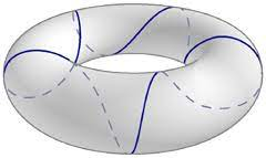
The Curvature and Geodesics of the Torus, Irons
The arc length equation gives us a distance metric
\[d(p,q)=\inf\{L(\gamma)\,|\,\gamma\in\mathcal{C}^{1}_{\operatorname{pw}}([0,1],\mathcal{M}),\\\gamma(0)=p,\gamma(1)=q\}\]
Curves which minimize this function are called geodesics.
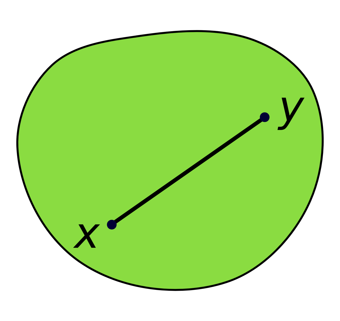
Convex Sets
A set \(X\subseteq\mathbb{R}^n\) is convex if \(\forall p,q\in X\), the line connecting \(p\) and \(q\) is contained in \(X\)
Geodesically Convex Sets
A set \(X\subseteq\mathcal{M}\) is geodesically convex (or g-convex) if \(\forall p,q\in X\), there is a unique length-minimizing geodesic (w.r.t. \(\mathcal{M}\)) connecting \(p\) and \(q\), which is completely contained in \(X\).
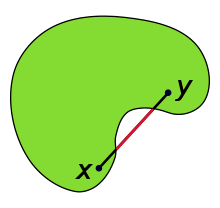
Convex Set, Wikipedia
Textbook references: Convex Optimization (Boyd 2004) and An Introduction to Optimization on Manifolds (Boumal 2023).
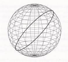
Some Sets Look Convex
(But Aren't)
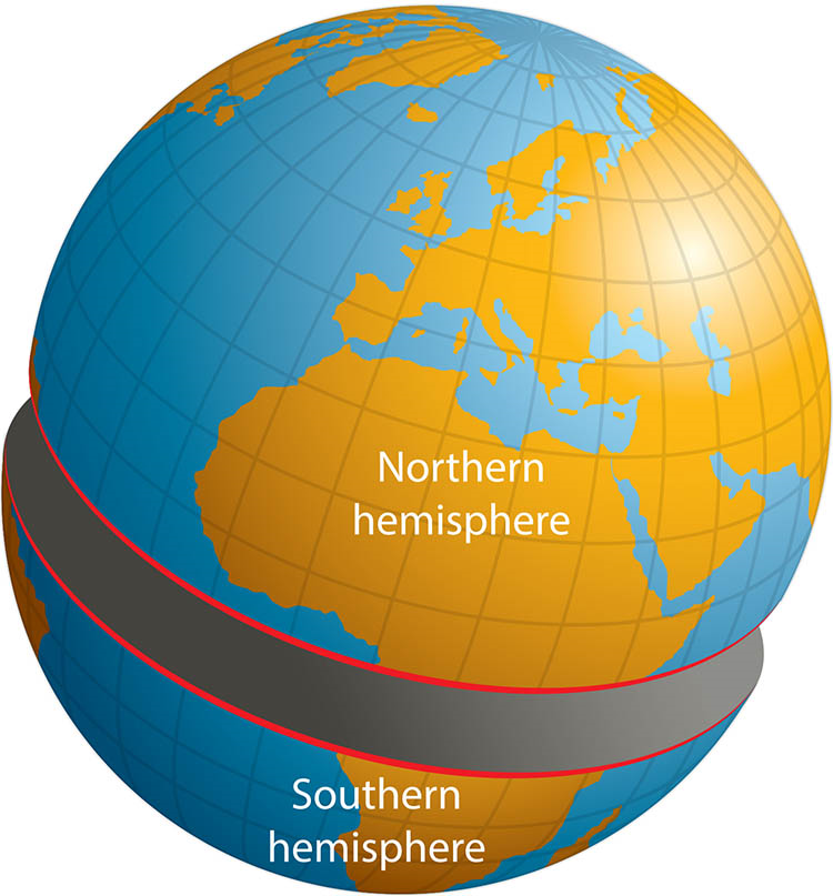
Sets can be convex in local coordinates, but not geodesically-convex on the manifold
Geodesics can go "the wrong way around"
Radius of convexity: how large can a set be and still be convex?
Which Continent Is Situated In All Four Hemispheres?, Junior
Convex Functions
A function \(f:X\to\mathbb{R}\) is convex if for any \(x,y\in X\) and \(\lambda\in[0,1]\), we have
\[f(\lambda x+(1-\lambda)y)\le\]
\[\lambda f(x)+(1-\lambda) f(y)\]
Geodesically Convex Functions
A function \(f:\mathcal{M}\to\mathbb{R}\) is geodesically convex if for any \(x,y\in \mathcal{M}\) and any geodesic \(\gamma:[0,1]\to\mathcal{M}\) such that \(\gamma(0)=x\) and \(\gamma(1)=y\), \(f\circ\gamma\) is convex

Hyperskill: Convex Functions, Patil
Part 3a
Methodology
Problem Statement
Configuration space \(\mathcal{Q}\) as a Riemannian manifold
\(\mathcal{M}\subseteq\mathcal{Q}\) is the set of collision free configurations, \(\bar{\mathcal{M}}\) its closure
The shortest path between \(p,q\in\bar{\mathcal{M}}\) is the solution to the optimization problem
\[\begin{array}{rl} \argmin & L(\gamma)\\ \textrm{subject to} & \gamma\in\mathcal{C}^{1}_{\operatorname{pw}}([0,1],\bar{\mathcal{M}})\\ & \gamma(0)=p\\ & \gamma(1)=q\end{array}\]
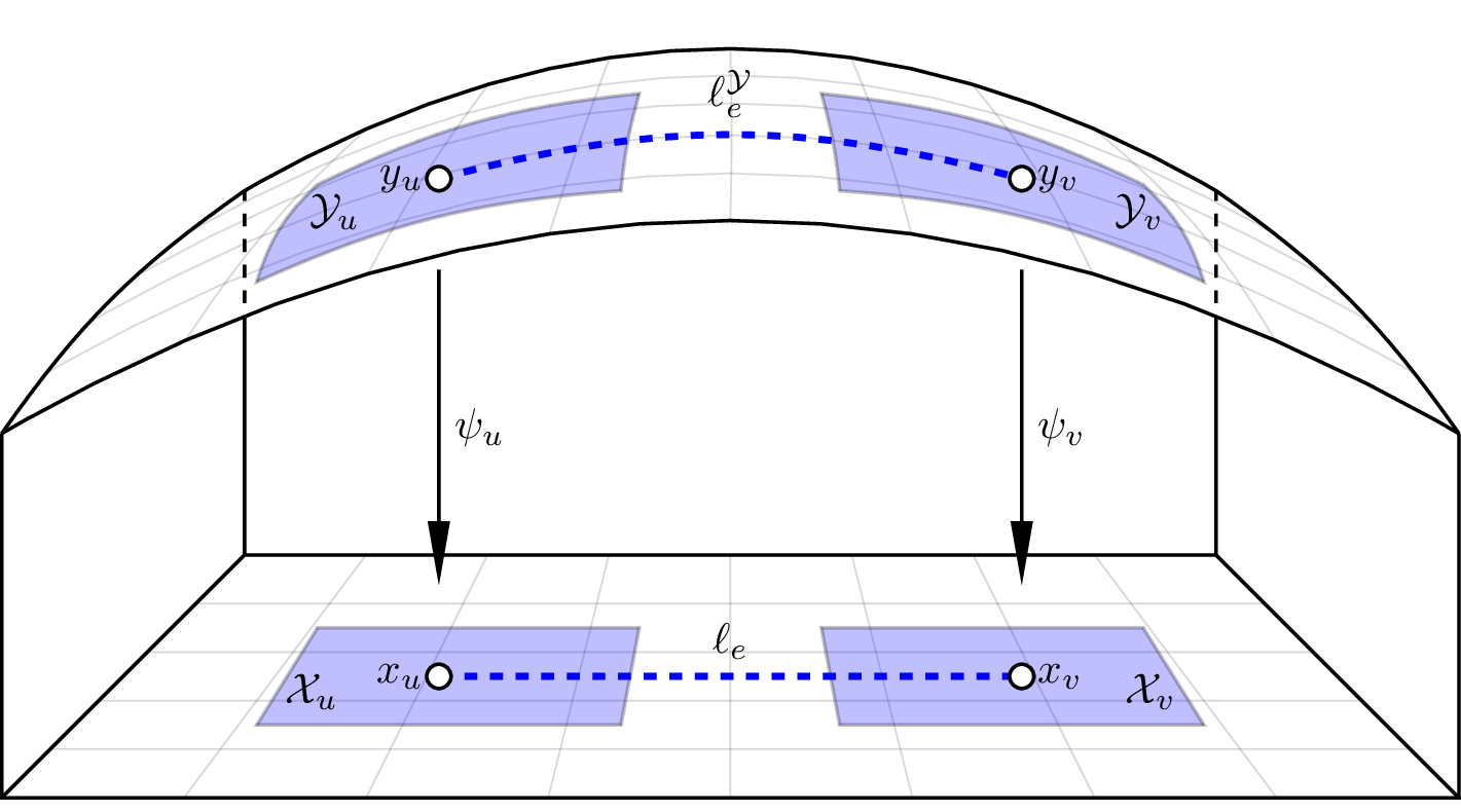
A Graph of Geodesically Convex Sets (GGCS)
A directed graph \(G=(V,E)\)
- For each vertex \(v\in V\), there is a g-convex set \(\mathcal{Y}_v\)
- For each edge \(e=(u,v)\in E\), there is a cost function \(\ell_e^\mathcal{Y}:\mathcal{Y}_u\times\mathcal{Y}_v\to\mathbb{R}\)
- \(\ell_e^\mathcal{Y}\) must be g-convex on \(\mathcal{Y}_u\times\mathcal{Y}_v\)
GCS
GGCS

Shortest Paths in GGCS
For each \(v\in V\), let \(\psi_v:\mathcal{Y}_v\to\mathbb{R}^n\) be a coordinate chart
Define \(X_v=\psi_v(\mathcal{Y}_v)\)
For each \(e=(u,v)\in E\), new edge cost:
\[\ell_e(x_u,x_v)=\ell_e^\mathcal{Y}(\psi_u^{-1}(x_u),\psi_v^{-1}(x_v))\]
If all \(X_v\) and \(\ell_e\) are convex, we have a valid GCS problem
Mixed-Integer Riemannian Optimization? No existing literature.
Better option: transform into a GCS problem
Transforming Back to a GCS
Nice Theoretical Results?
- There is a shortest path \(\gamma\) connecting \(p\) to \(q\) through \(\bar{\mathcal{M}}\) such that
- \(\gamma\) is piecewise geodesic
- Each geodesic segment is contained in some \(\bar{X}_u\)
- \(\gamma\) passes through each \(\bar{X}_u\) at most once
- Ensures that a shortest path is feasible for GGCS
- Formal equivalence of GGCS and transformed GCS problem
When is it Convex?
Have to consider the curvature of the manifold.

Positive curvature
E.g. \(S^n,\operatorname{SO}(3),\operatorname{SE}(3)\)
Negative curvature
E.g. Saddle, PSD Cone \(\vphantom{S^n}\)
Zero curvature
E.g. \(\mathbb R^n, \mathbb T^n\)
?
Zero-Curvature is Still Useful
- All 1-dimensional manifolds
- Continuous revolute joints
- \(\operatorname{SO}(2)\), \(\operatorname{SE}(2)\)
- Products of flat manifolds
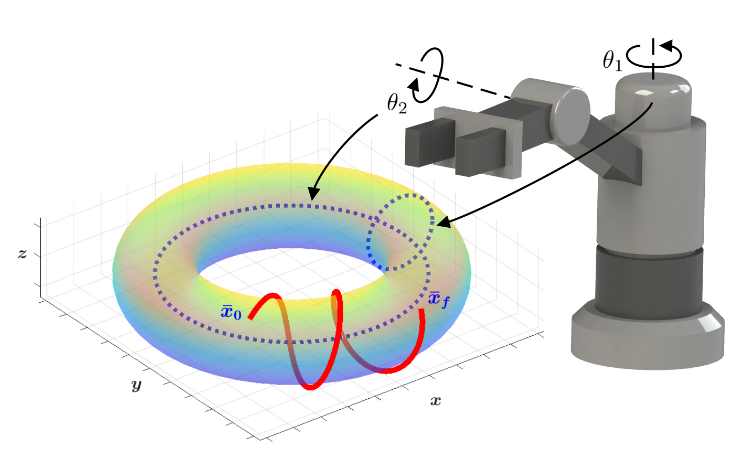
Fetch Robot Configuration
Space: \(\operatorname{SE}(2)\times \mathbb{T}^3\times \mathbb{R}^7\)
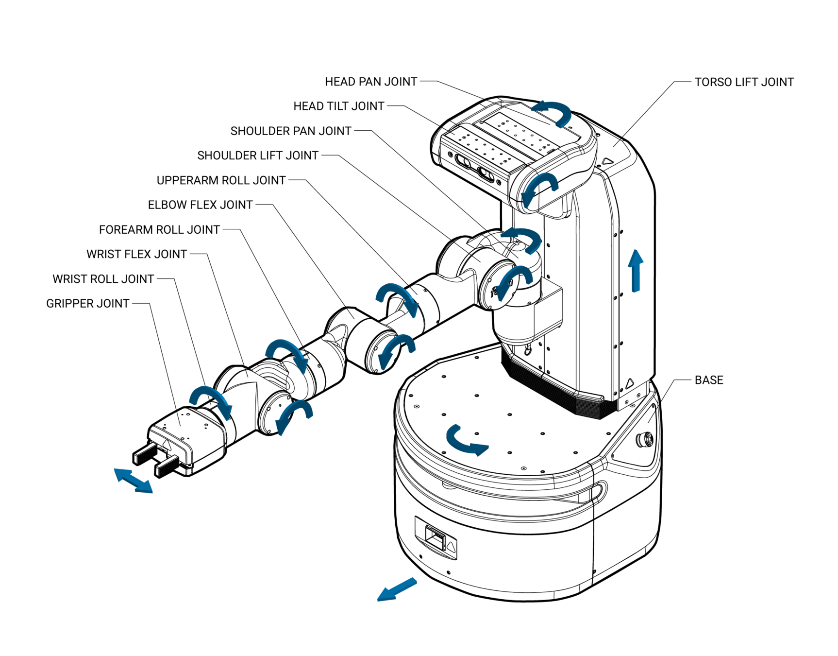
Trajectory Control for Differential Drive Mobile Manipulators, Karunakaran and Subbaraj
Part 3b
Experimental Results
"Asteroids" World
Square with opposite edges identified
Configuration Space: \(\mathbb{T}^2\)
Planar Arm
A robot arm with 5 continuous revolute joints in the plane
Configuration Space: \(\mathbb{T}^5\)
(No self collisions)

Path Length Comparison

Part 3c
Beyond Flat Manifolds
Why is Positive Curvature Bad?

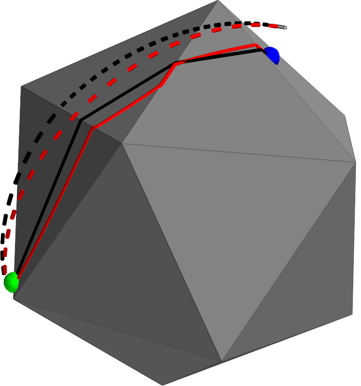
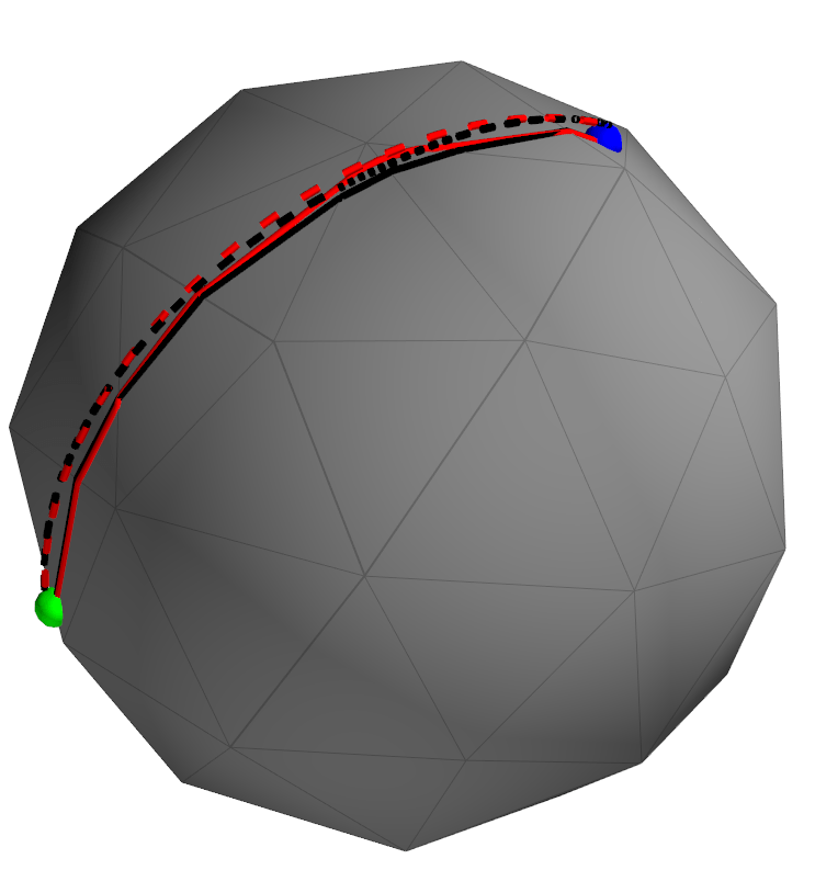
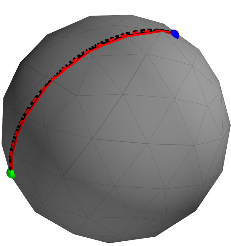
Planning on PL Approximations
Black: Shortest path on PL approximation
Red: Shortest path on sphere
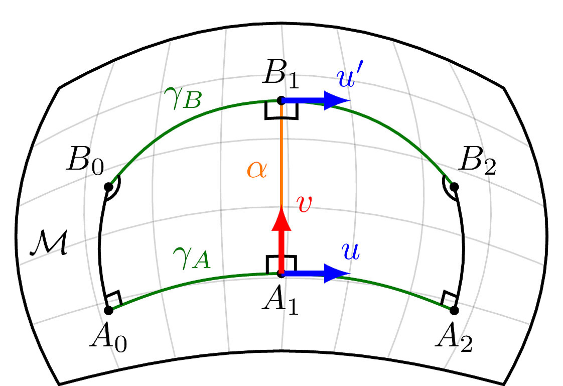
Rough Bounds on Approximation Error
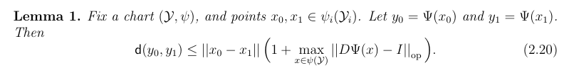
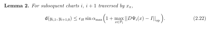
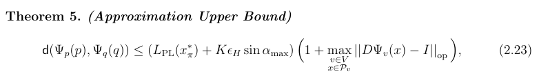
Intuition: How much does the Jacobian of the chart vary?
Intuition: The amount we can "slip" along the boundary also depends on the Hausdorff distance \(\epsilon_H\) between the manifold and its triangulation, as well as the angle \(\alpha_{\operatorname{max}}\) between adjacent charts.
Intuition: The error grows additively with the number of sets traversed in the optimal path.
Focusing on SO(3)/SE(3)
Recall that \(\operatorname{SE}(3)\) is just \(\operatorname{SO}(3)\times\mathbb R^3\)
Three representations for \(\operatorname{SO}(3)\):
- Euler angles (\(S^1\times S^1\times S^1\))
- Axis-angle (\(S^2\times S^1\))
- Unit quaternions (\(S^3\))
Notation: \(S^n\) is the \(n\)-sphere. (\(S^1\) is the circle, \(S^2\) is the ordinary sphere in 3D space, etc.)
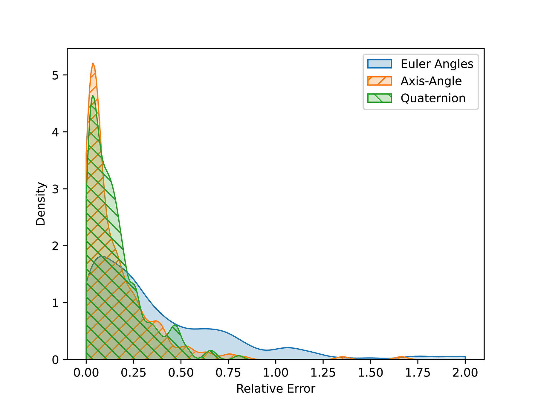
Numerical Comparison
Randomly sample \(n\) start and goal pairs, plan between them with each approximation.
Compute the true distance, and explore the error distribution.
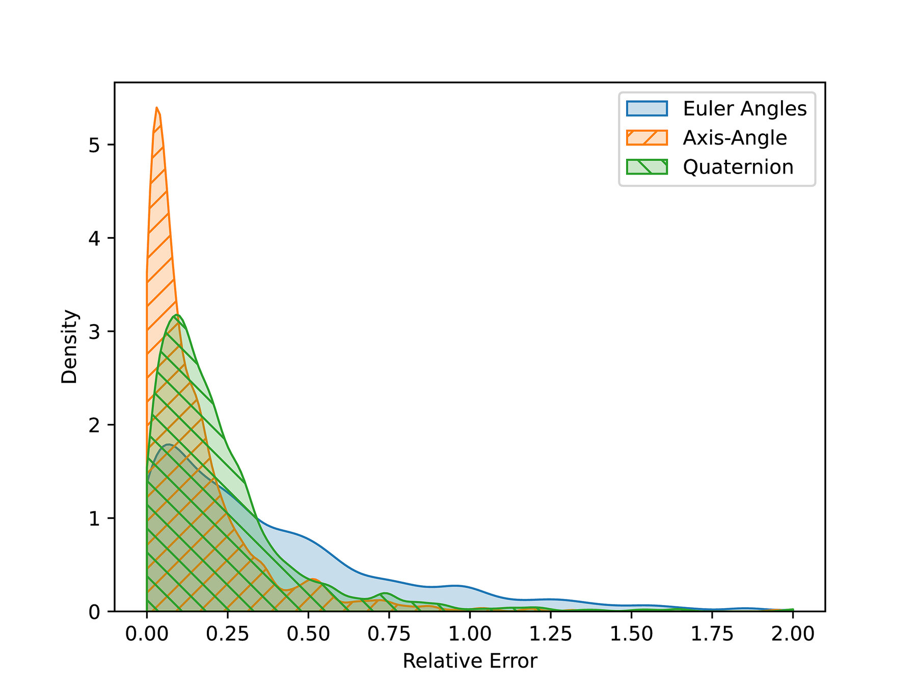
(Low Resolution Quaternion Approximation)
(High Resolution Quaternion Approximation)
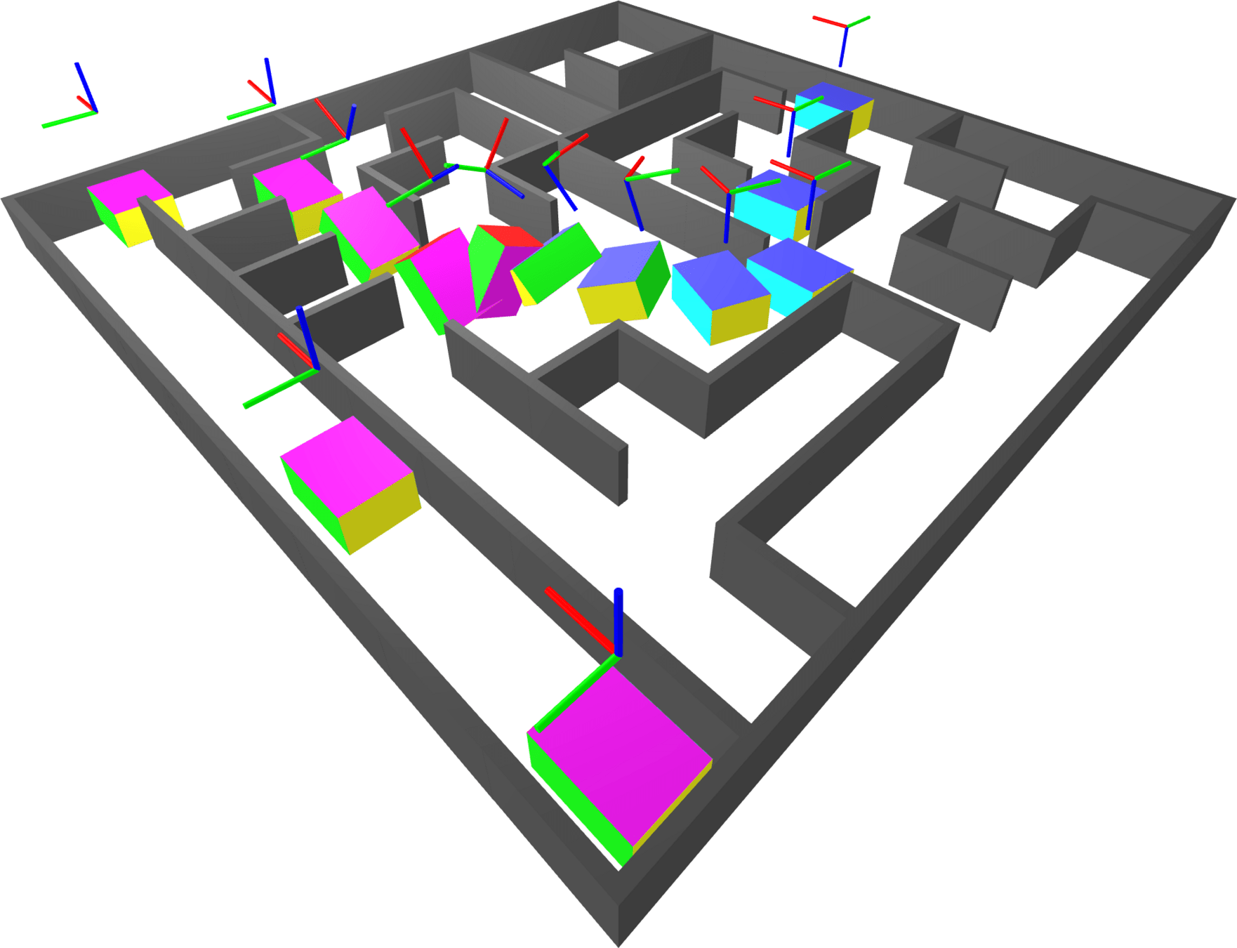
Shortest Paths in the Maze
Sample path between a start/goal pair.
The large gap in the center gives room for the block to reorient itself.
Part 4
What Comes Next?
Kinematic Constraints
Learning the Metric of Task Constraint Manifolds for Constrained Motion Planning, Zha et. al.
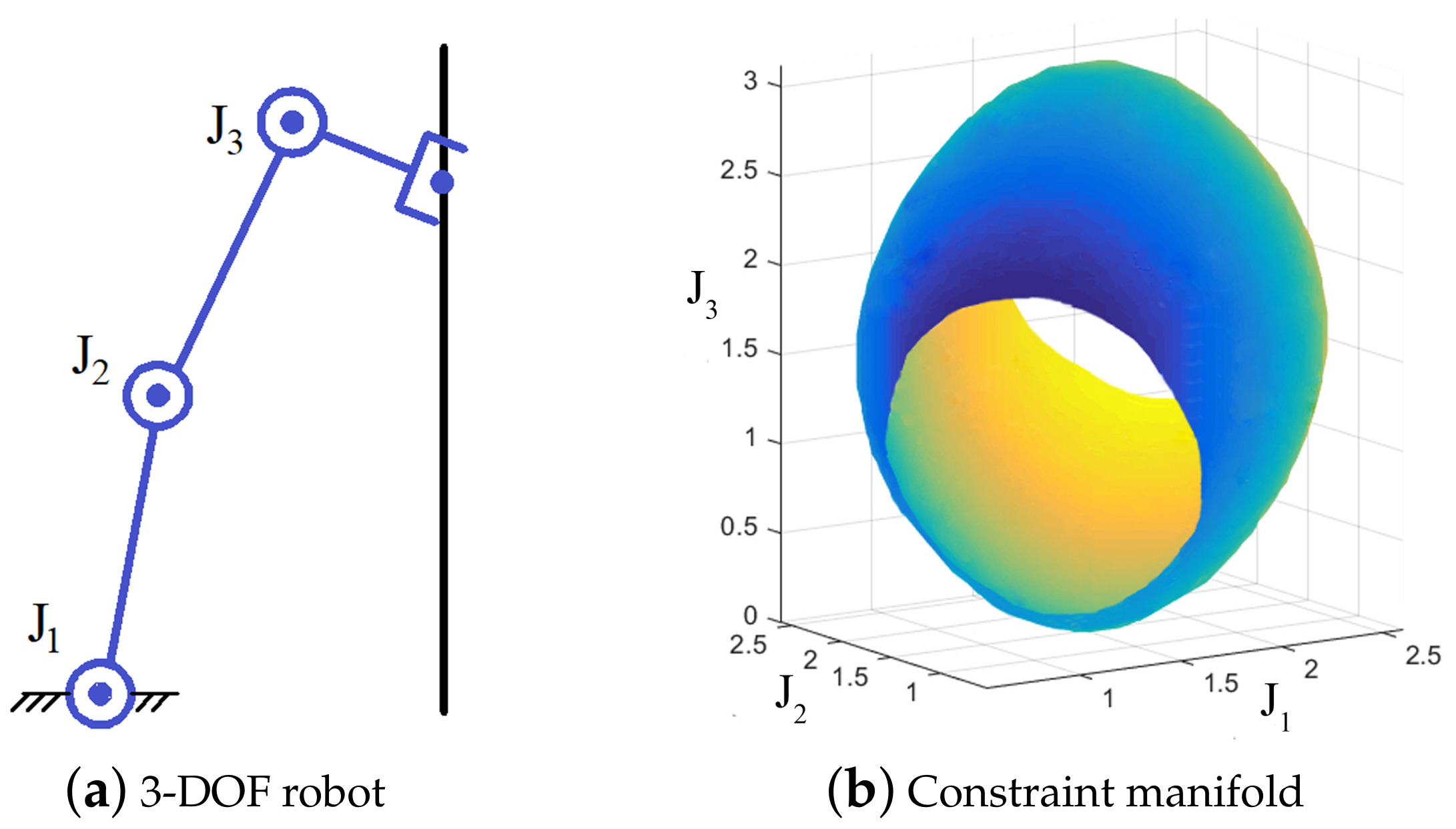
Parametrizing the Constraint Manifold

Constrained Bimanual Planning with Analytic Inverse Kinematics, Thomas Cohn, Seiji Shaw, Max Simchowitz, Russ Tedrake
Bimanual Manipulation
Constrained Bimanual Planning with Analytic Inverse Kinematics, Thomas Cohn, Seiji Shaw, Max Simchowitz, Russ Tedrake
Nonconvex Objectives
Planning Shorter Paths in Graphs of Convex Sets by Undistorting Parametrized Configuration Spaces, Shruti Garg, Thomas Cohn, and Russ Tedrake
Nonconvex Objectives
Planning Shorter Paths in Graphs of Convex Sets by Undistorting Parametrized Configuration Spaces, Shruti Garg, Thomas Cohn, and Russ Tedrake

Non-Euclidean Motion Planning with Graphs of Geodesically-Convex Sets
Robot Locomotion Group
Thomas Cohn, Mark Petersen, Max Simchowitz, Russ Tedrake
RQE Presentation - February 12, 2025
RQE Presentation
By tcohn


