


Théo Dumont
PhD student in optimal transport & geometry @ Université Gustave Eiffel
Théo Dumont
D., Lacombe, Vialard. Learning Monge maps with constrained drifting models, preprint, 2026.
joint work with T. Lacombe and F.-X. Vialard
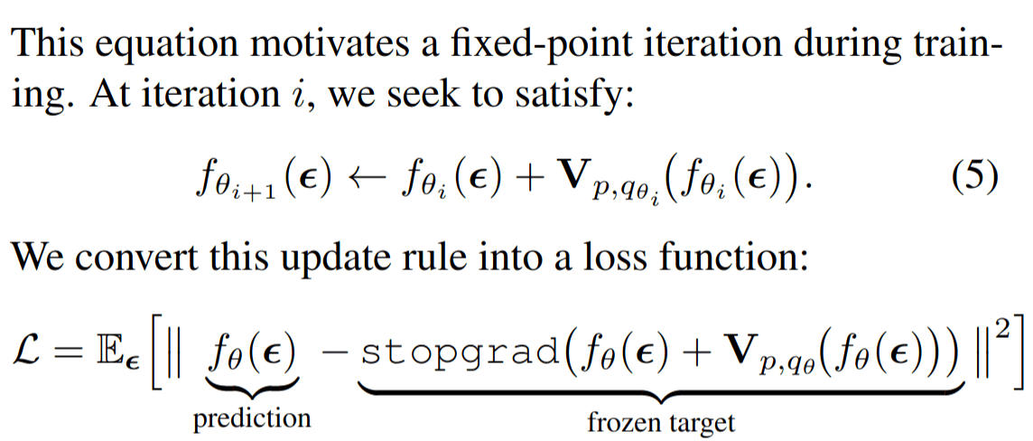
Université Gustave Eiffel, LIGM
Let \(\mu_0,\gamma\in\mathcal P(\mathbb R^d)\) with finite 2nd-order moment.
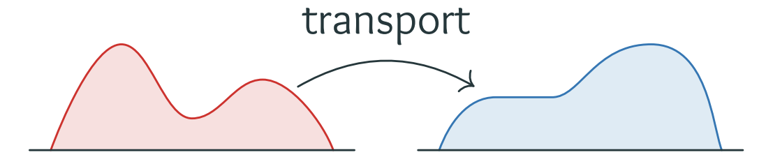
Optimal transport: the Monge problem
\(|\!\det dT^{-1}|\rho_0 \circ T^{-1}\)
[Monge, 1781], [Kantorovitch, 1942], [Brenier, 1987]
Definition. (OT problem)
If \(\mu_0\) has a density, then there is a unique solution to (OT), and it is the unique map pushing \(\mu_0\) onto \(\gamma\) that writes \(T^\star=\nabla \phi\) with \(\phi:\mathbb R^d\to\mathbb R\) convex.
Theorem. (Brenier)
\(T^\star\in\)
the set of OT/Monge maps
Finding the OT map: existing methods
Let \(\mu_0,\gamma\in\mathcal P(\mathbb R^d)\) with finite 2nd-order moment.
Methods (non-exhaustive):
In practice, we have samples \(\widehat\mu_n=\frac1n\sum_{i=1}^{n}\delta_{x_i}\) and \(\widehat\gamma_n=\frac1n\sum_{i=1}^{n}\delta_{y_i}\), and we want an estimate \(\widehat T_n\) of \(T^\star\).
Can we find a class of measures such that the estimation of the OT map is not dim. cursed? (gradient flows??)
?
[D, Lacombe, Vialard, 2026]
Finding the OT map: our method
Definition. (OT problem)
\(T^\star\) is the gradient of a convex function \(\phi\).
Theorem. (Brenier)
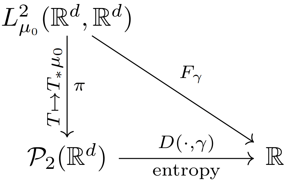
Let \(D:\mathcal P(\mathbb R^d)\times \mathcal P(\mathbb R^d)\to\mathbb R_{\geq0}\) such that
\(D(\mu,\nu)=0\iff\mu=\nu\).
Our new problem.
Then \(T_*\mu_0=\gamma\iff D(T_*\mu_0,\gamma)=0\).
1. The optimality constraint.
2. The pushforward constraint.
(it is a closed convex cone)
Let \(H\) be some Hilbert space and let \(F:H\to \mathbb R\).
Say I want to find
Gradient flows in Hilbert spaces
Proof.
The gradient flow of some function \(F:H\to\mathbb R\) is a solution \(x_t\) of
starting at some \(x_0\in H\), for all \(t\geq0\).
Definition. (Gradient flow)
Assume that \(F\) is \(\lambda\)-convex with \(\lambda>0\). Then \(x_t\) converges to the unique \(x^\star\) at an exponential rate: \[\|x_t-x^\star\|^2\leq e^{-\lambda t}\|x_0-x^\star\|^2.\]
Theorem. (convergence of gradient flow)
Finding a convex functional \(D\)
\(\displaystyle D(\mu,\gamma)\coloneqq \int_{\mathbb R^d}\log\frac{\mathrm d\mu}{\mathrm d\gamma}\,\mathrm d\mu=\int_{\mathbb R^d} V\,\mathrm d\mu+\int_{\mathbb R^d}\log\mu\,\mathrm d\mu \)
entropy
potential
Write \(\gamma=e^{-V}\,\mathrm dx\). Define the relative entropy (or KL divergence):
if \(\mu\ll\gamma\), else \(\infty\).
If \(V\) is \(\lambda\)-convex on \(\mathbb R^d\), then \(D(\cdot,\gamma)\) is \(\lambda\)-convex on \(\mathcal P_2(\mathbb R^d)\) along generalized geodesics, that is, along all curves \[\mu_t=[(1-t)T+tS]_*\mu_0\quad\text{for all }T,S\in K.\]
Theorem. [Ambrosio, Gigli, Savaré, 2005]
If \(V\) is \(\lambda\)-convex on \(\mathbb R^d\), then \(F_\gamma\) is \(\lambda\)-convex on \(K\), that is, along all curves \[(1-t)T+tS\quad\text{for all }T,S\in K.\]
Corollary. [D., Lacombe, Vialard, 2026]
Find a function \(D\) such
that \(F_\gamma\) is convex on \(K\)?
?
We need to stay in \(K\)!
!
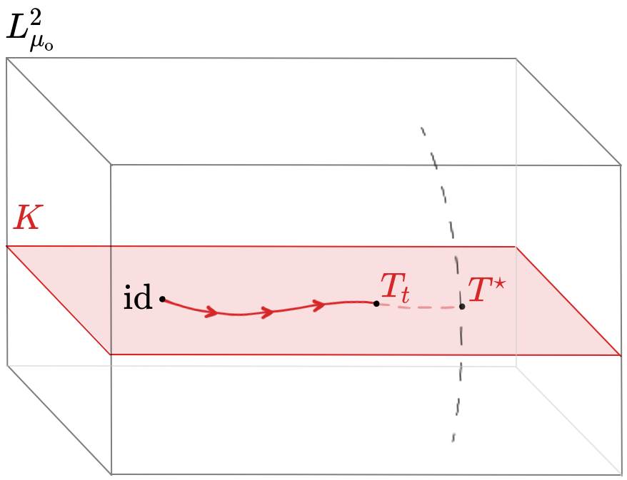
A gradient flow in the set of transport maps?
starting at \(T_0=\operatorname{id}\), for all \(t\geq0\).
The increment \(-\operatorname{grad} F_\gamma(T)\) does not make \(T_t\) stay in \(K\) (except in 1D situations).
Some intuition:
\[-\operatorname{grad} F_\gamma(T)=-\nabla_{\text{W}}D(T_*\mu_0)\circ T,\]where \(\nabla_{\text{W}}D(\mu)=\nabla\frac{\delta D}{\delta\mu}(\mu)\), and
\(\nabla p\circ \nabla q\) is not a gradient in general.
[Lavenant, Santambrogio, 2022]
So in order to find , we might consider
the gradient flow of \(F_\gamma\):
A constrained gradient flow in the set of transport maps
Let \(\mu_0\in\mathcal P(\mathbb R^d)\) with a density, let \(\gamma=e^{-V}\in\mathcal P(\mathbb R^d)\) with \(V\) \(\lambda\)-convex, \(\lambda>0\), and let \(D\) be the relative entropy wrt \(\gamma\). Then the constrained gradient flow:
starting at \(T_0=\operatorname{id}\),
\(\circ\) admits a solution \(t\mapsto T_t\) of time-regularity \(H^1\)
\(\circ\) it converges exponentially fast to the OT map between \(\mu_0\) and \(\gamma\): \[\|T_t-T^\star\|^2_{\mu_0}\leq Ce^{-2\lambda t}\|\operatorname{id}-T^\star\|^2_{\mu_0}.\]
Theorem. [D., Lacombe, Vialard, 2026]
Recall the set of optimal maps
Its (Clarke) tangent cone is
(where \(T=\nabla\phi\))
Key ingredients:
\(\circ\) \(K\) is closed and convex in the Hilbert space \(L^2_{\mu_0}(\mathbb R^d,\mathbb R^d)\)
\(\circ\) to build a solution: approximate the flow by a discrete implicit scheme
(see GMM/JKO) in the Hilbert space \(L^2_{\mu_0}(\mathbb R^d,\mathbb R^d)\) for the convex and l.s.c. functional \(F_\gamma+\imath_K\)
\(\circ\) to prove convergence: similar to standard proofs of convergence of g.f. for convex functionals
[Ambrosio, Gigli, Savaré, 2005], [Rossi, Savaré, 2006]
Definition. (OT problem)
Our new problem.
Everything holds for a slightly broader class of functionals:
\(\circ\) only need convexity along a subset of generalized geodesics, those that write \[\mu_t=[(1-t)T+T^\star]_*\mu_0\](i.e. that have \(\mu_0\) as anchor point and \(\gamma\) as endpoint.
\(\circ\) still convergence results for mere convexity (not \(\lambda\)-convexity)
starting at \(T_0=\operatorname{id}\), for all \(t\geq0\).
A constrained gradient flow in the set of transport maps
[D, Lacombe, Vialard, 2026]
Recall the constrained gradient flow:
To implement this computationally, one needs to:
1. discretize the flow in time (either with an explicit or an implicit Euler scheme)
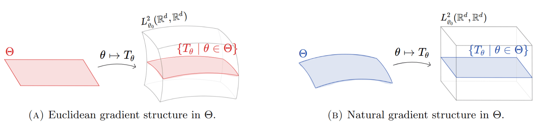
2. parameterize the set \(K\) with some parameterization \(K_\theta\coloneqq\{T_\theta\mid\theta\in\Theta\}\subset K\),
where \(\theta\mapsto T_\theta\in K\) is e.g. a \(\nabla\)ICNN (Input Convex Neural Network)
This yields:
Implementing the constrained gradient flow
We compare the results with the standard gradient descent/flow approach:
(explicit constr. GD)
(implicit constr. GD)
Constrained gradient descent.
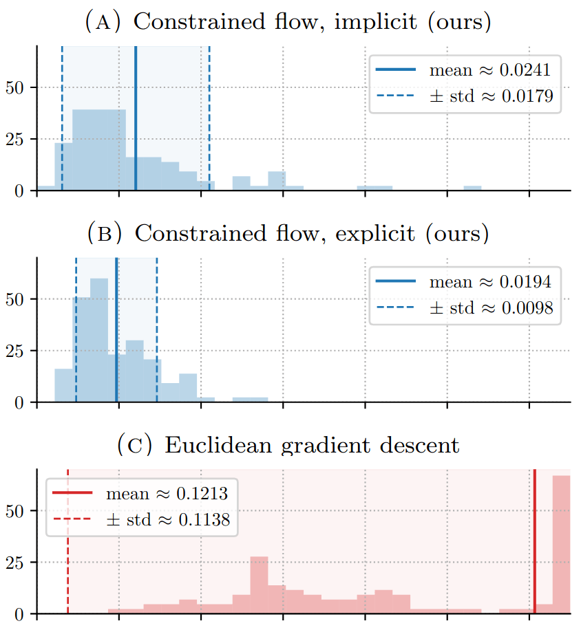
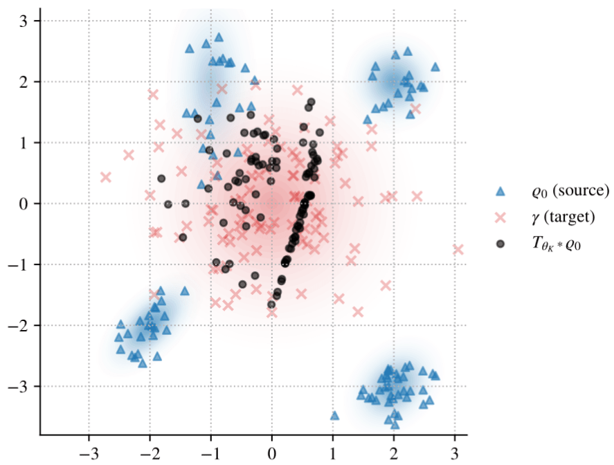
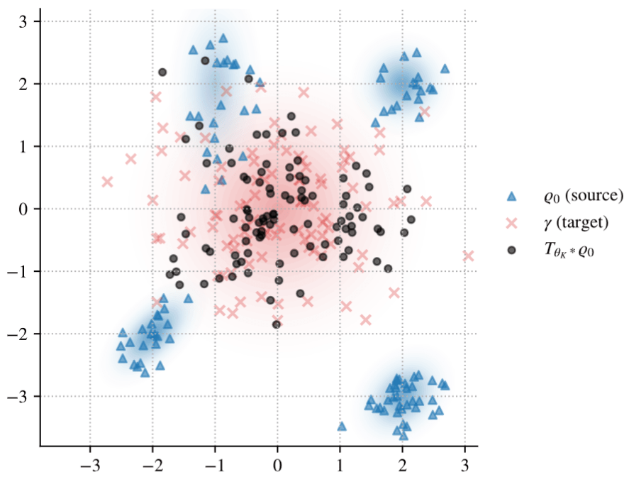
Numerical PoC
Fig. 2: Distribution of \(\operatorname{MMD}_{\text{ED}}(\widehat T_*\mu_0,\gamma)\).
Fig. 1: Visualization of \(\widehat T_*\mu_0\) and \(\gamma\).
Link 1: natural gradient descent schemes
This flow on \(\Theta\) is the gradient flow of \(\theta\mapsto F_\gamma(T_\theta)=D(T_\theta{}_*\mu_0,\gamma)\) with respect to the pullback of the flat \(L^2_{\mu_0}\)-metric by the mapping \(\theta\mapsto T_\theta\), i.e. a \(L^2_{\mu_0}\)-natural gradient flow (under standard regularity assumptions).
Proposition. [D., Lacombe, Vialard, 2026]
In the limit \(\tau\to0\), the parameterized flow becomes
Link 2: drifting models
[Deng et al., 2026]
Differences:
\(\circ\) they are not constrained to optimal maps
\(\circ\) not the same choice of vector field \(\mathbf V\)
\(\circ\) we have convergence guarantees
Let \(v_{\theta_k}\coloneqq -\nabla_{\text{W}}D(T_{\theta_k}{}_*\mu_0)\).
(explicit constr. GD)
D., Lacombe, Vialard. Learning Monge maps with constrained drifting models, preprint, 2026.
Ambrosio, Gigli, Savaré (2005). Gradient flows: in metric spaces and in the space of probability measures
Brenier (1987). Décomposition polaire et réarrangement monotone des champs de vecteurs
Deng, Li, Li, Du, He (2026). Generative Modeling via Drifting.
Dumont, Lacombe, Vialard (2026). Learning Monge maps with constrained drifting models.
Kantorovich (1942). On the translocation of masses.
Monge (1781). Mémoire sur la théorie des déblais et des remblais.
Rossi, Savaré (2006). Gradient flows of non convex functionals in Hilbert spaces and applications.
Villani (2008). Optimal transport: old and new.
slides available at https://slides.com/theodumont/monge-constrained-cs
•
•
•
•
•
•
•
•
References
Thank you!
By Théo Dumont
Talk about learning Monge maps with constrained drifting models (https://arxiv.org/abs/2603.25182https://arxiv.org/abs/2603.25182https://arxiv.org/abs/2603.25182


