Lecture 11 : K-means and Gaussian Mixture Models
Assoc. Prof. Yuan-Sen Ting
Astron 5550 : Advanced Astronomical Data Analysis
Logistics
Homework Assignment 4 due next Friday,11:59pm
Group Project 2 - Project Selection - feedback found on Carmen
Group Project 2 - Presentation - April 18
Group Project 2 - Report - April 28 (no deferment)
Plan for Today :
K-means
Gaussian Mixture Models
Expectation-Maximization Algorithm
Information Criterion
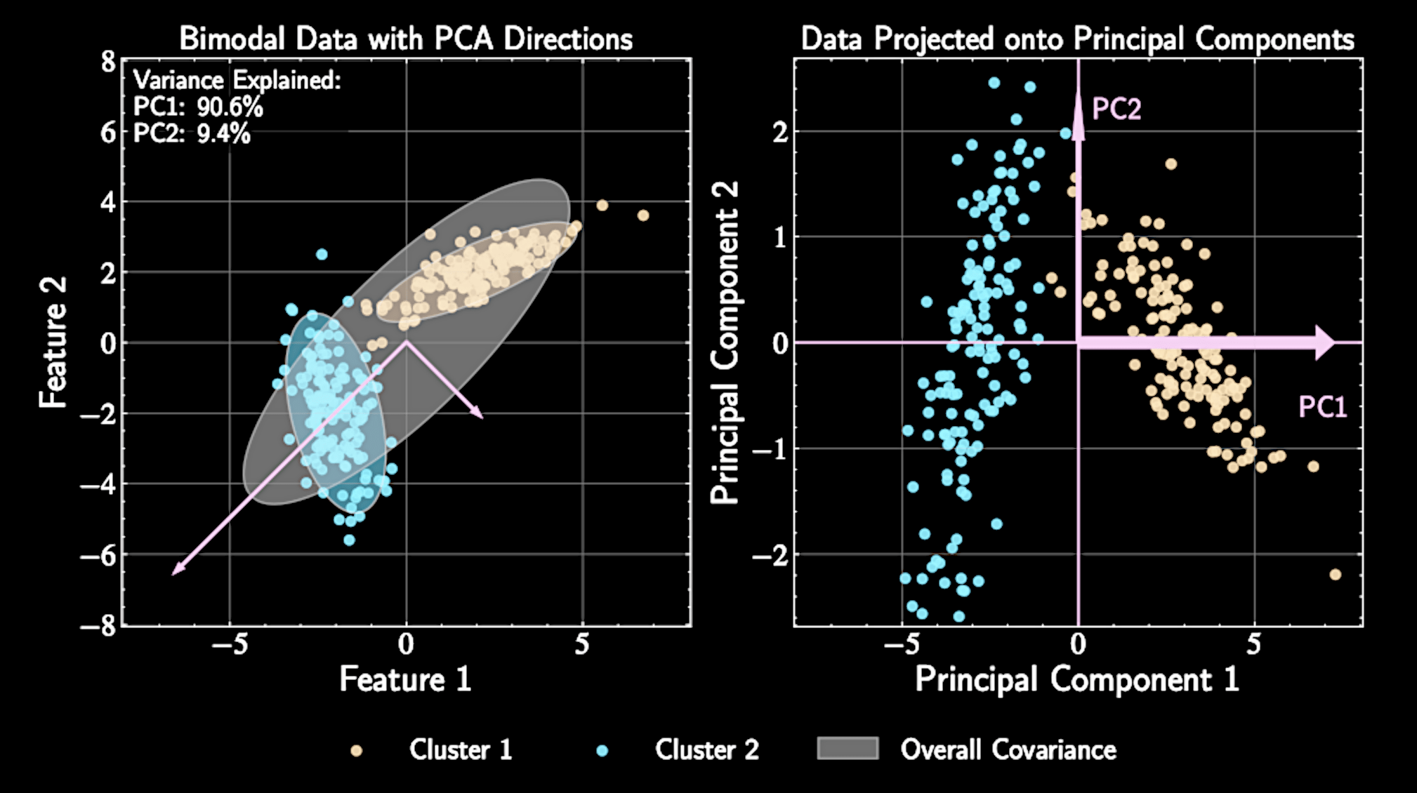
From Dimension Reduction to Clustering
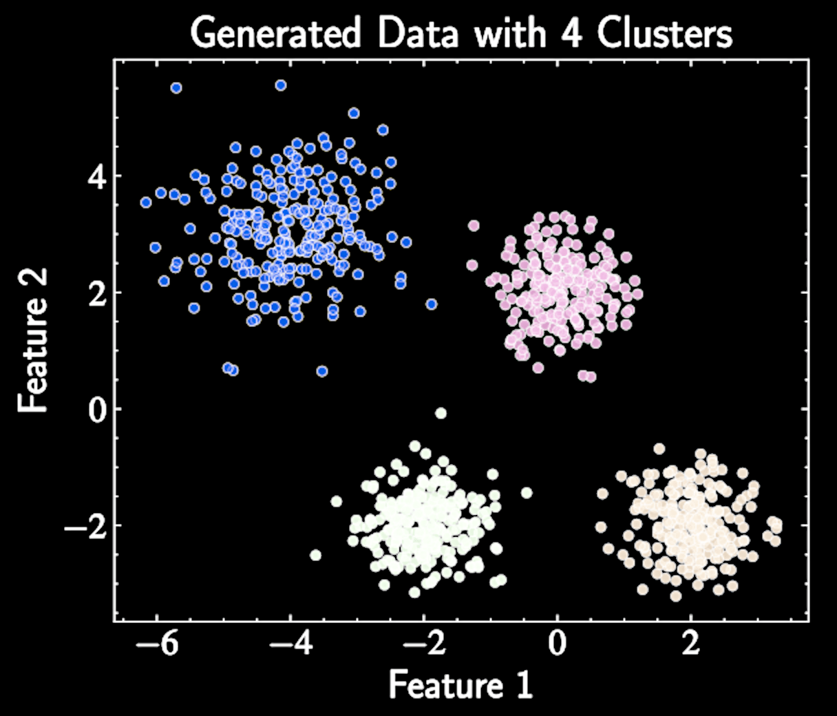
Clustering identifies natural groupings in unlabeled data
Dimension reduction: continuous representations preserving important variations
Clustering: discrete partitioning based on similarity measures
Both techniques uncover structure but with different approaches.
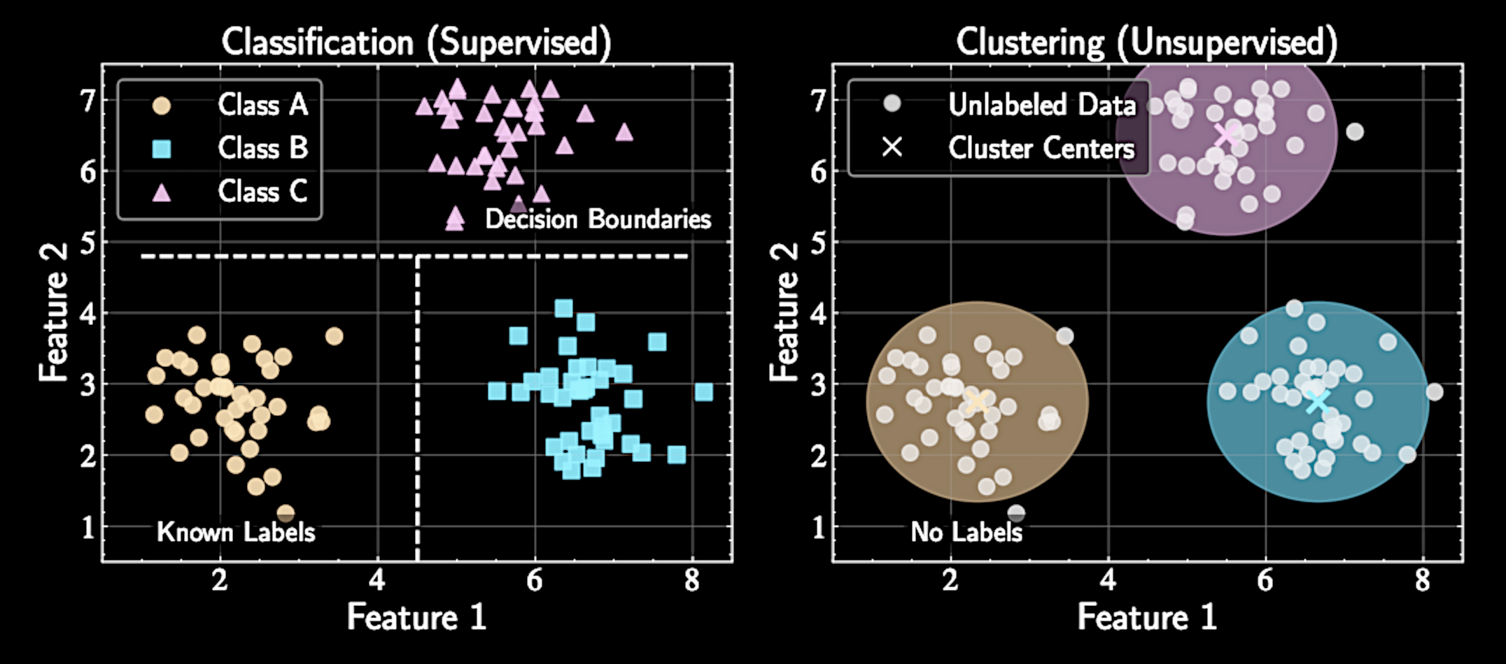
Clustering versus Classification
Classification requires labeled training data and finds decision boundaries between known categories
Clustering allows exploration without preconceived categories of what should exist
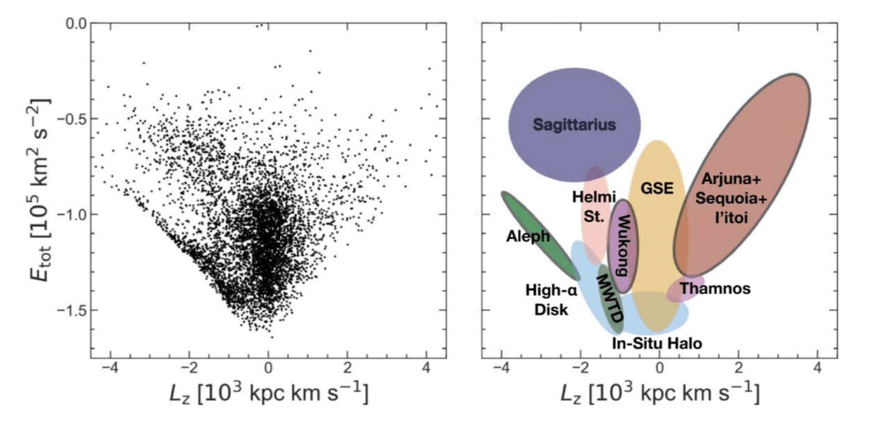
Naidu et al. 2020
Clustering versus Classification
Classification requires labeled training data and finds decision boundaries between known categories
Clustering allows exploration without preconceived categories of what should exist
However, without ground truth labels, evaluating clustering quality becomes more subjective
The appropriate number of clusters is often unclear and may depend on the scientific question
Approaches to Clustering
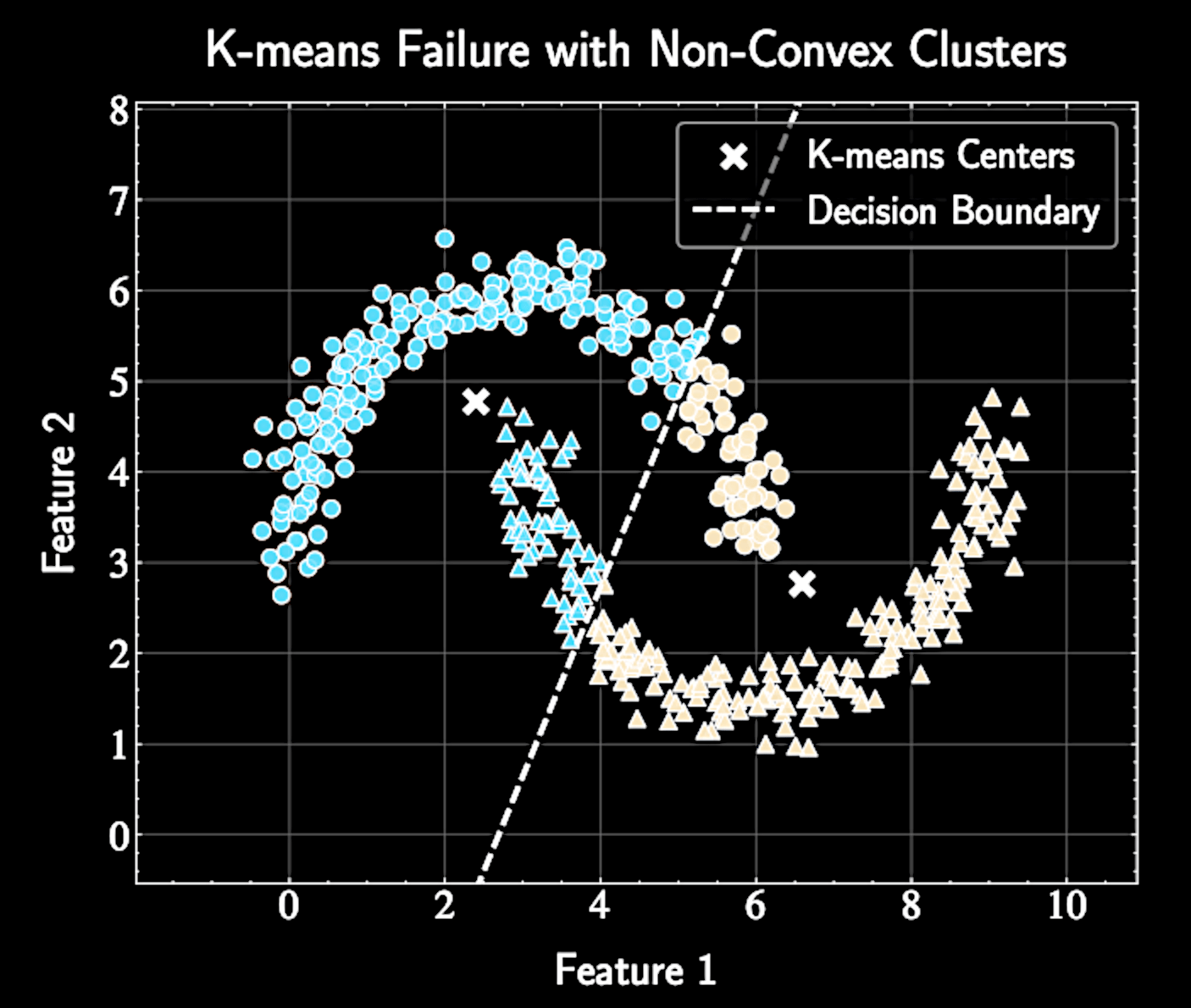
K-means partitions data by minimizing distance to cluster centers but assumes spherical clusters
Gaussian Mixture Models (GMMs) model data as a mixture of several Gaussian distributions
K-means is computationally efficient and scalable to large astronomical datasets
GMMs align with Bayesian approach to probabilistic inference and better quantify uncertainty in clustering
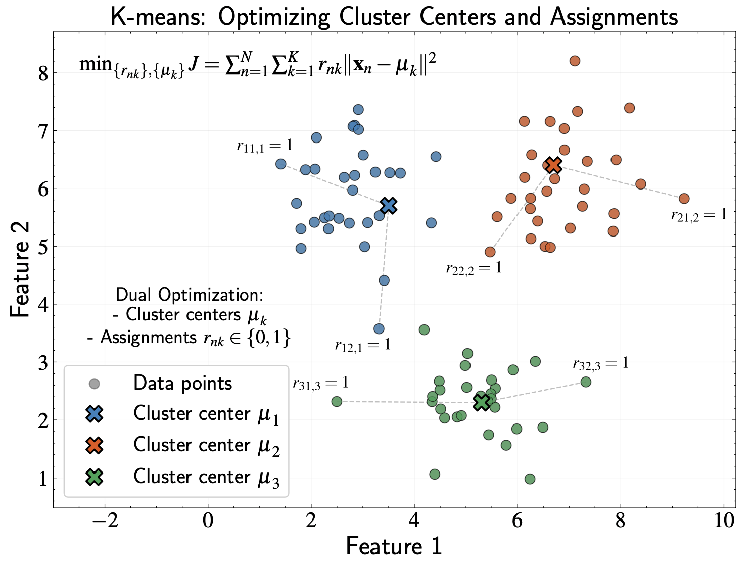
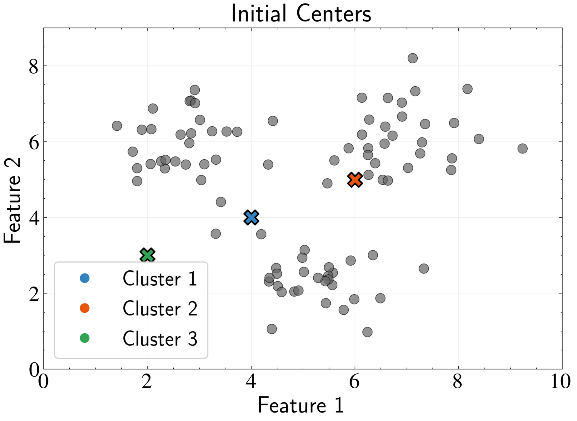
K-means: Core Concept
K-means partitions data into K clusters with optimal cluster centers
Data points are assigned to the cluster whose center is closest to them
We must optimize two parameter sets simultaneously: cluster centers and point assignments
Mathematical Notation
Dataset: \( {\mathbf{x}_1, \mathbf{x}_2, \ldots, \mathbf{x}_N} \), where each \( \mathbf{x}_n \) is D-dimensional
Cluster centers: \( {\boldsymbol{\mu}_1, \boldsymbol{\mu}_2, \ldots, \boldsymbol{\mu}_K} \)
Binary indicator variables: \( r_{nk} \in \{0, 1\} \).
Constraint: \( \sum_{k=1}^K r_{nk} = 1 \)
Each data point must belong to exactly one cluster
("hard assignment")
K-means Objective Function
We minimize:
Each point contributes exactly one non-zero term
(its assigned cluster)
Two parameter sets to optimize simultaneously: centers \( \boldsymbol{\mu}_k \) and assignments \( r_{nk} \)
J = \sum_{n=1}^N \sum_{k=1}^K r_{nk} |\mathbf{x}_n - \boldsymbol{\mu}_k|^2
The Chicken-and-Egg Problem
If we knew cluster centers, assignments would be trivial (assign to nearest center)
If we knew assignments, optimal centers would be straightforward (mean of assigned points)
Binary constraint alone creates combinatorial complexity with \( K^N \) possible assignment combinations
Standard gradient descent methods are impractical
Expectation Maximization Algorithm: Key Insight
Optimizing both cluster centers and assignments simultaneously is difficult
Optimizing one parameter set while keeping the other fixed is straightforward
EM follows a "zig-zag" path through parameter space toward a minimum
Complex optimization problem decomposes into sequence of simpler analytical problems
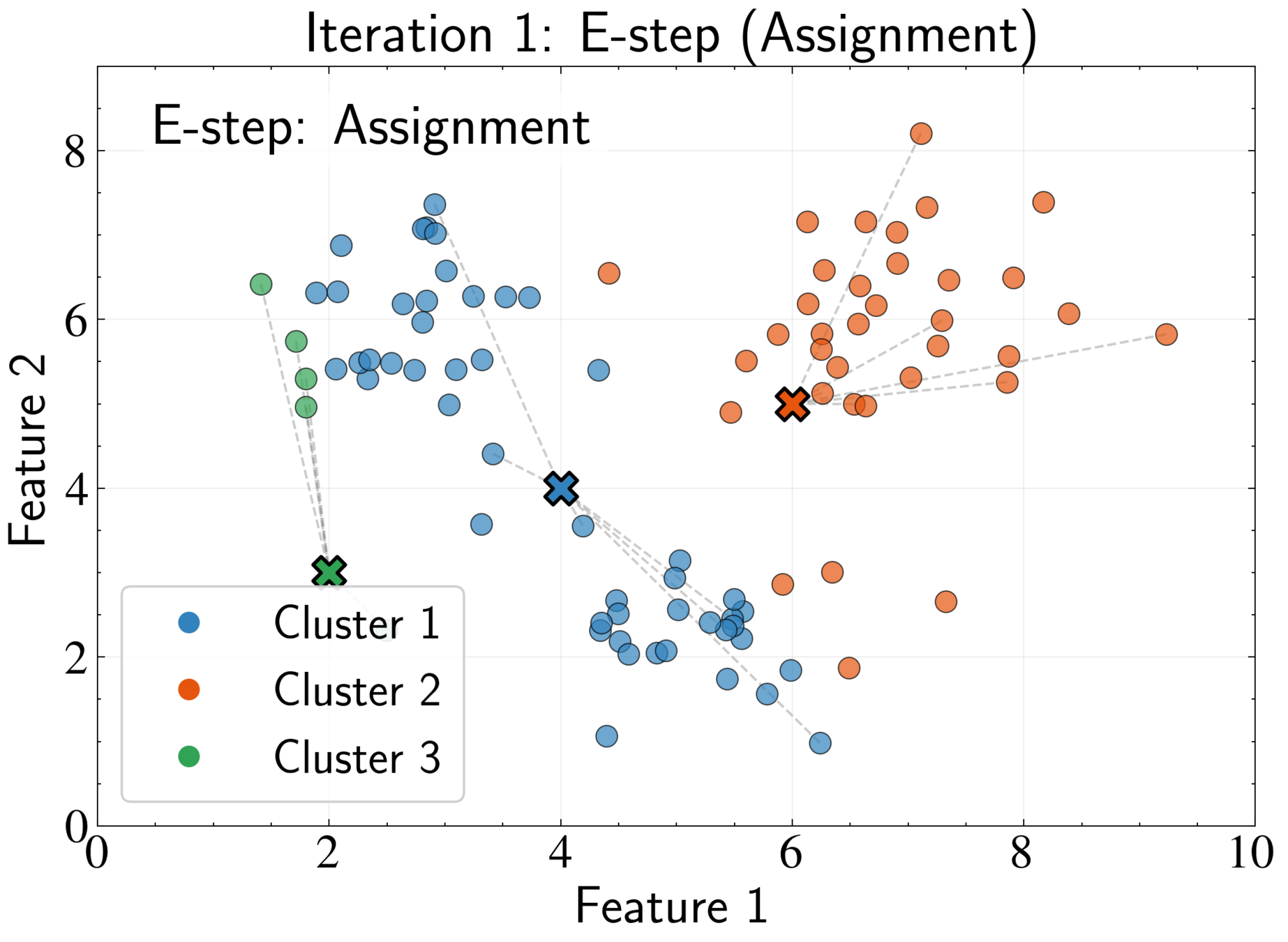
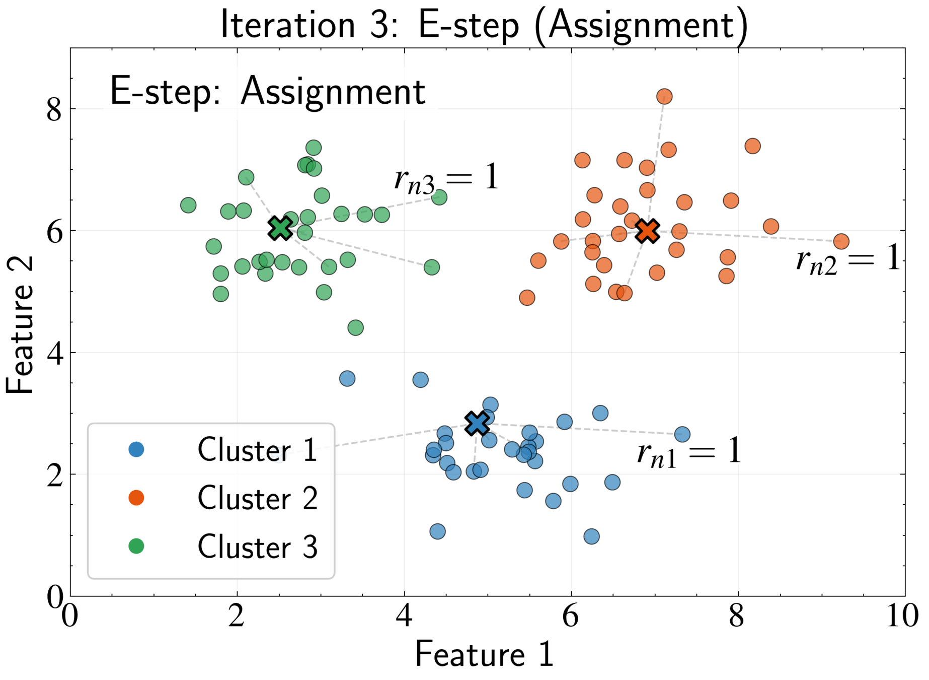
EM Algorithm for K-means: E-step
Fix cluster centers \( \boldsymbol{\mu}_k \) and optimize assignments \( r_{nk} \)
Optimal assignment:
Assign each point to its nearest cluster center
J = \sum_{n=1}^N \sum_{k=1}^K r_{nk} |\mathbf{x}_n - \boldsymbol{\mu}_k|^2
r_{nk} = \begin{cases}
1 & \text{if } k = \arg\min_{j} |\mathbf{x}_n - \boldsymbol{\mu}_j|^2 \\
0 & \text{otherwise}
\end{cases}
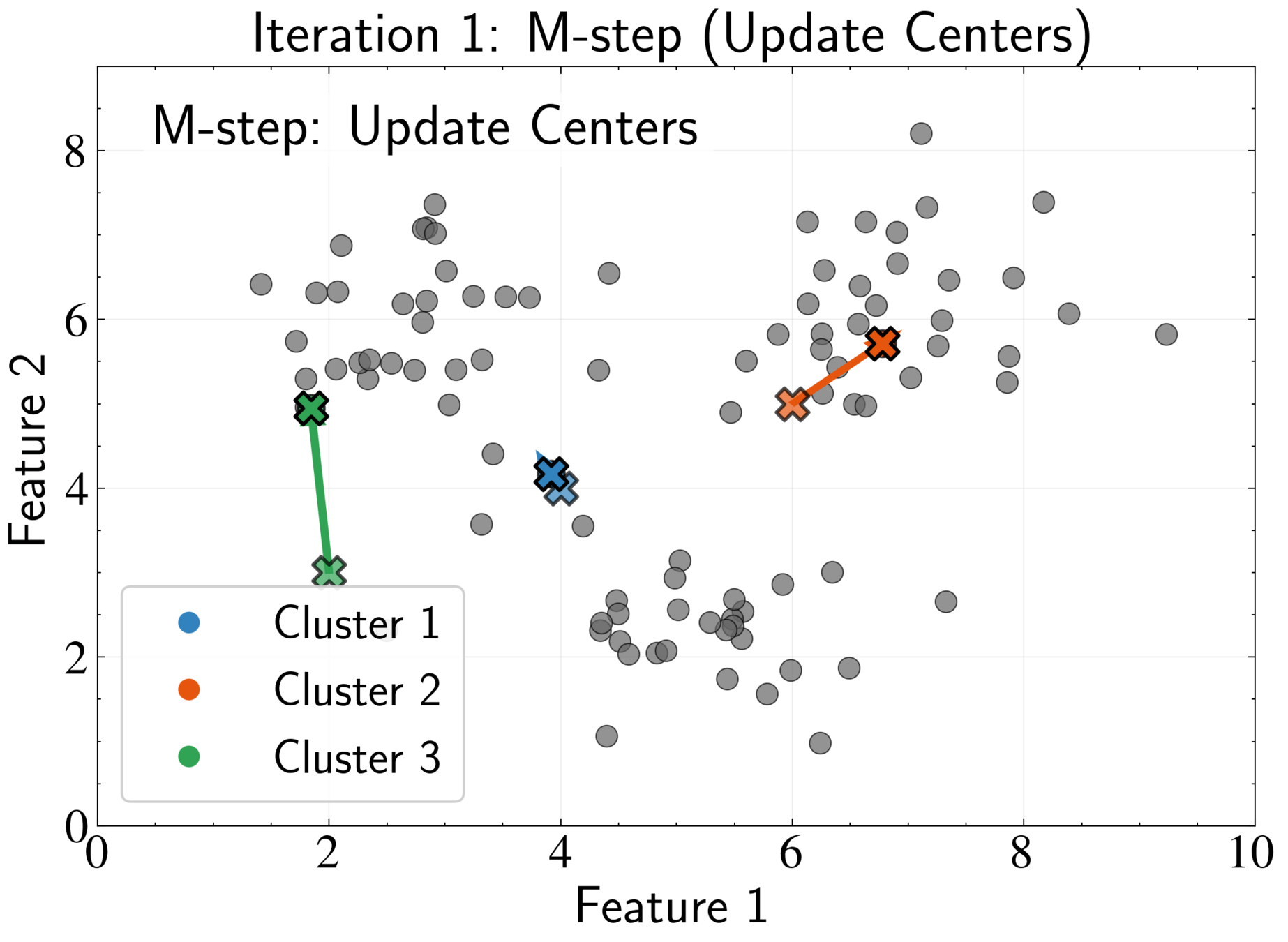
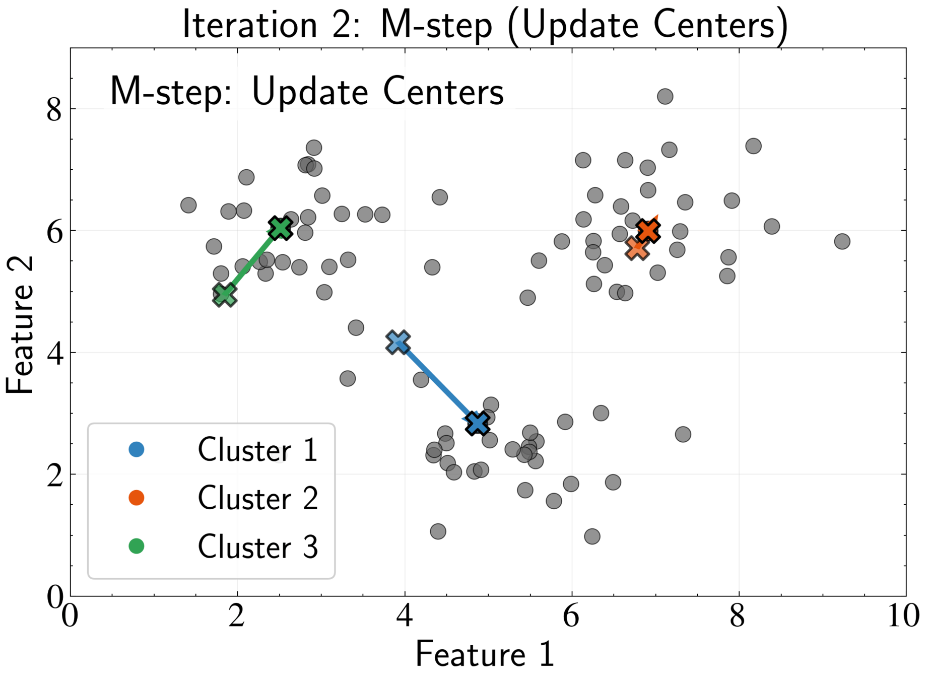
EM Algorithm for K-means: M-step
Fix assignments \( r_{nk} \) and optimize cluster centers \( \boldsymbol{\mu}_k \)
Take gradient with respect to \( \boldsymbol{\mu}_k \):
J = \sum_{n=1}^N \sum_{k=1}^K r_{nk} |\mathbf{x}_n - \boldsymbol{\mu}_k|^2
\frac{\partial J}{\partial \boldsymbol{\mu}_k} = \sum_{n=1}^N r_{nk} \frac{\partial}{\partial \boldsymbol{\mu}_k} |\mathbf{x}_n - \boldsymbol{\mu}_k|^2
= \sum_{n=1}^N r_{nk} (-2)(\mathbf{x}_n - \boldsymbol{\mu}_k)
EM Algorithm for K-means: M-step
Take gradient with respect to \( \boldsymbol{\mu}_k \):
J = \sum_{n=1}^N \sum_{k=1}^K r_{nk} |\mathbf{x}_n - \boldsymbol{\mu}_k|^2
\frac{\partial J}{\partial \boldsymbol{\mu}_k} = -2 \sum_{n=1}^N r_{nk} \mathbf{x}_n + 2 \boldsymbol{\mu}_k \sum_{n=1}^N r_{nk} = 0
\boldsymbol{\mu}_k = \frac{\sum_{n=1}^N r_{nk} \mathbf{x}_n}{\sum_{n=1}^N r_{nk}}
Optimal center is the mean of all points assigned to that cluster
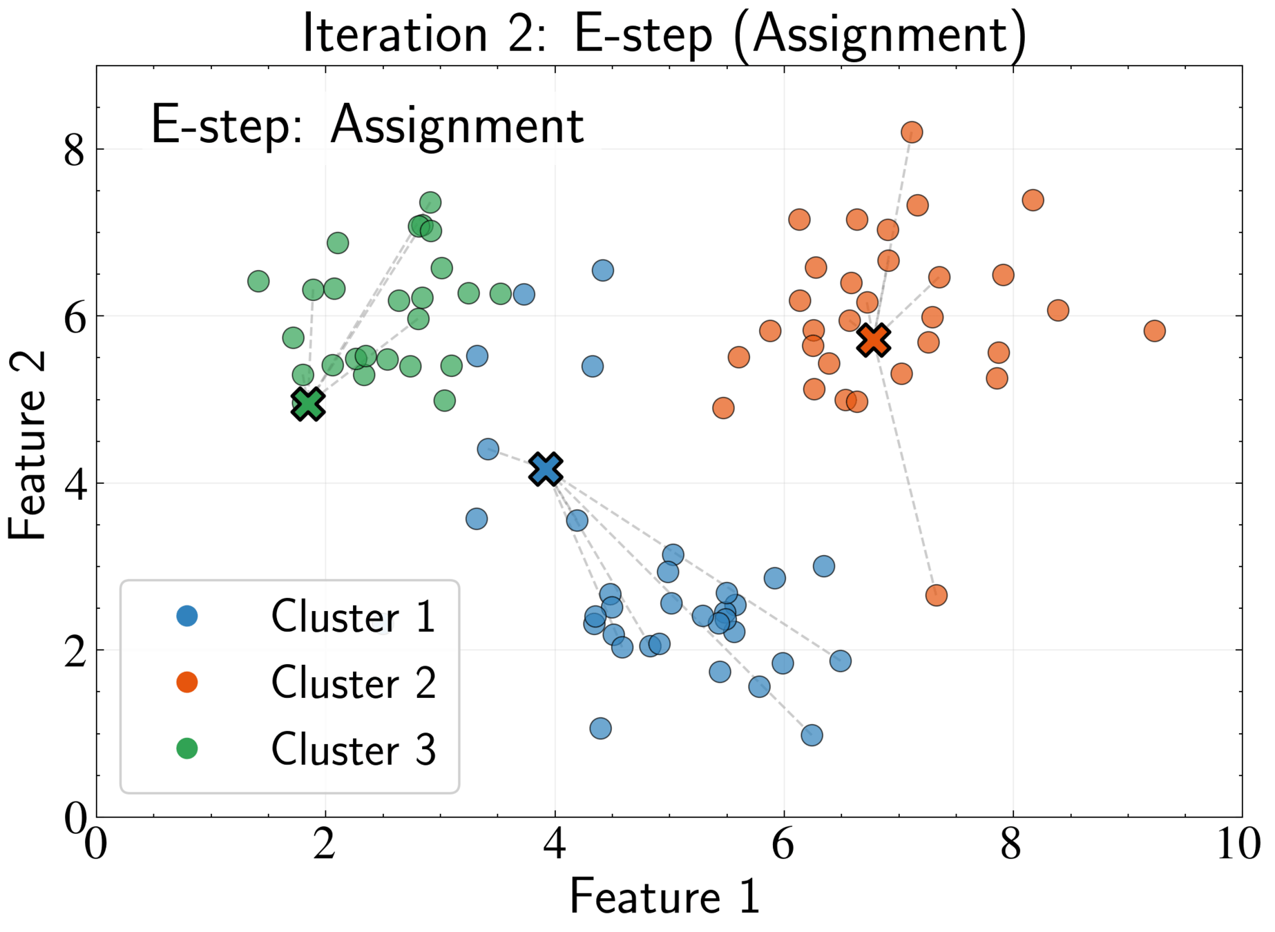
EM Algorithm for K-means
Repeat E-step and M-step until convergence
Convergence occurs when assignments no longer change significantly
EM Algorithm for K-means
Repeat E-step and M-step until convergence
Convergence occurs when assignments no longer change significantly
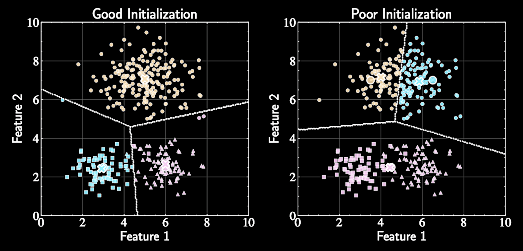
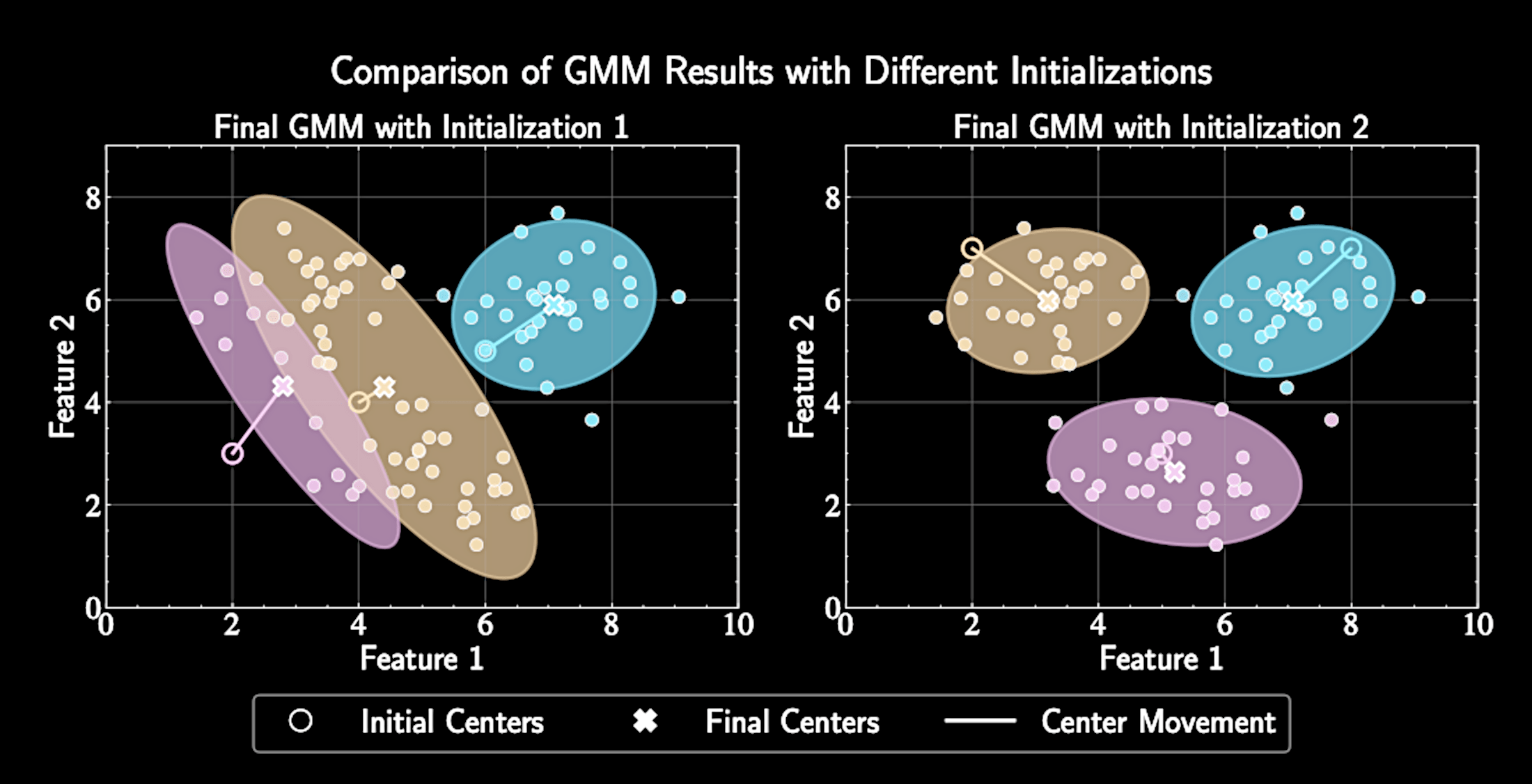
Algorithm converges to a local minimum, not necessarily the global minimum
Final solution depends on initial centers, need multiple runs.
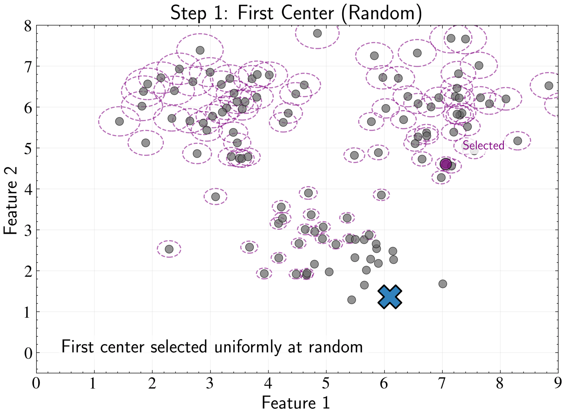
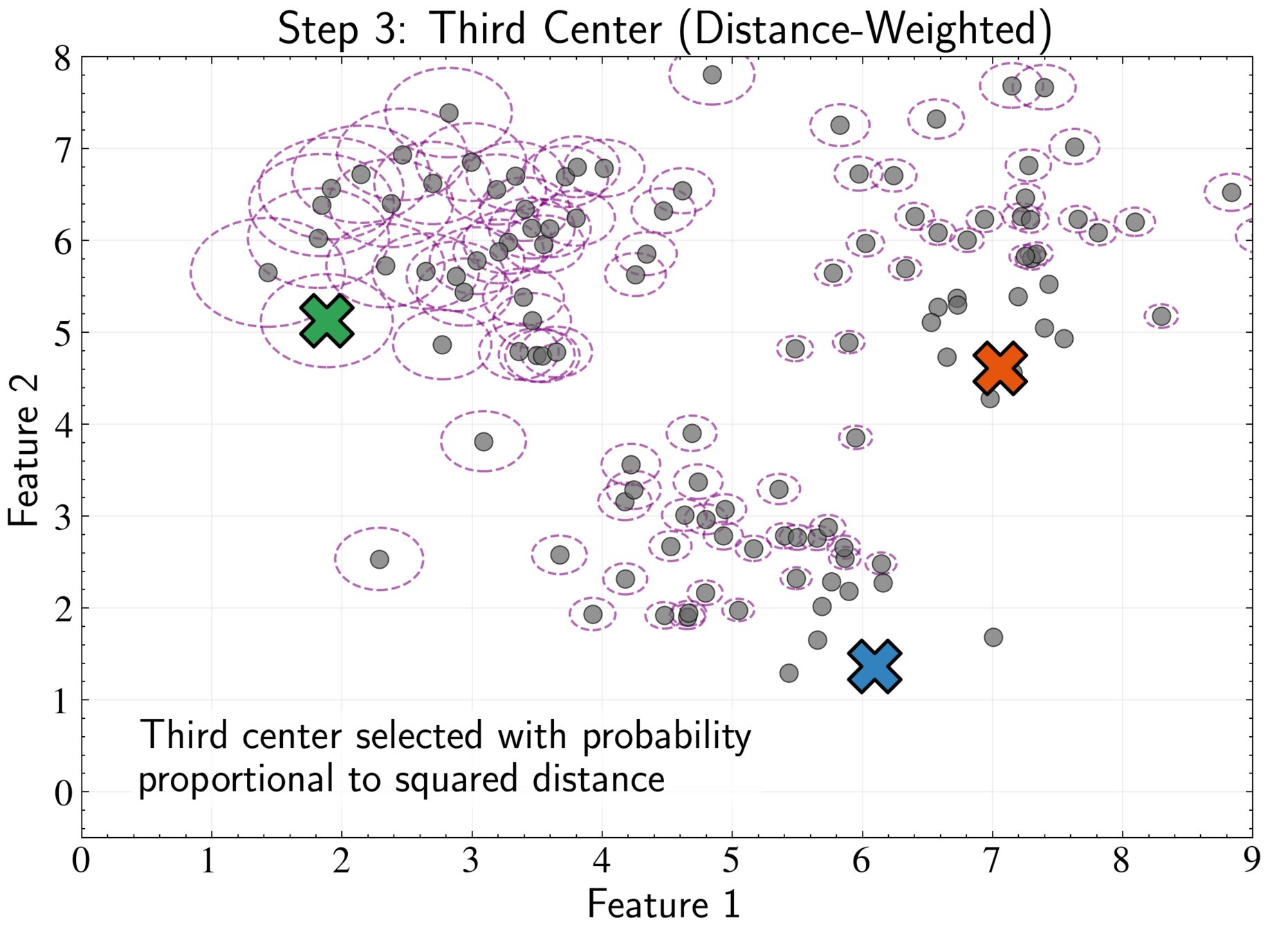
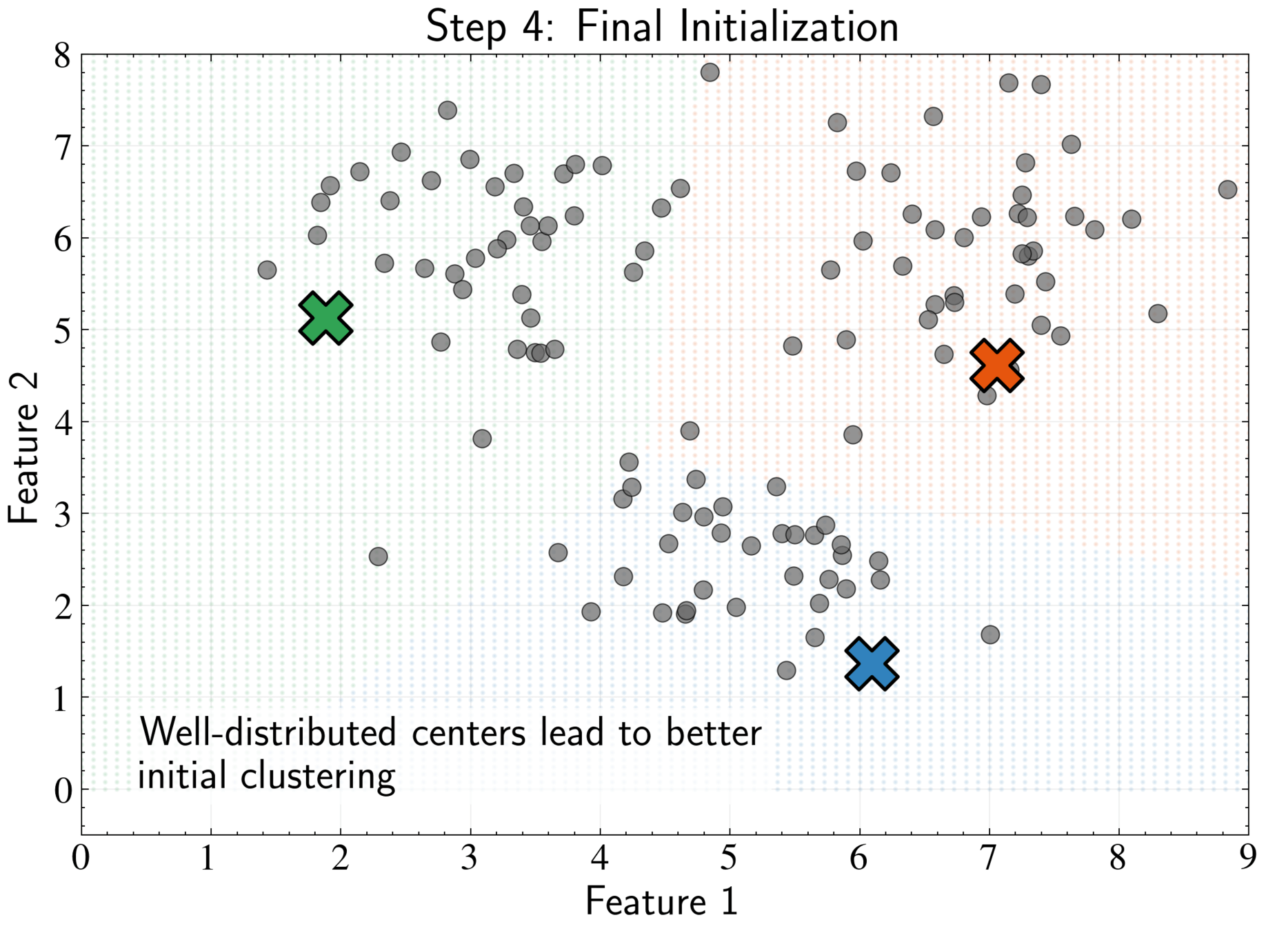
K-means++ Initialization Strategy
More systematic approach to choosing initial cluster centers
Select first center uniformly: \( P(\boldsymbol{\mu}_1 = \mathbf{x}_n) = \frac{1}{N} \) for all n
For each data point, compute minimum distance to existing centers: \( \)
D(\mathbf{x}_n) = \min_{j \in \{1,2,\ldots,m\}} |\mathbf{x}_n - \boldsymbol{\mu}_j|^2
K-means++ Initialization Strategy
Select next center with probability proportional to \( D(\mathbf{x}_n)^2\):
Maximize minimum distance between centers while respecting data density
Repeat until all K centers are chosen, then proceed with standard K-means
P(\boldsymbol{\mu}_{m+1} = \mathbf{x}_n) = \frac{D(\mathbf{x}_n)^2}{\sum_{i=1}^N D(\mathbf{x}_i)^2}

Inductive Biases of Clustering with K-Means
Spherical covariances (same for all clusters)
Hard assignments of points to clusters
Gaussian Mixture Models (GMMs) relax these restrictive assumptions for more flexible clustering
J = \sum_{n=1}^N \sum_{k=1}^K r_{nk} |\mathbf{x}_n - \boldsymbol{\mu}_k|^2
Computational Complexity of K-means
Distance calculation complexity: \(\mathcal{O}(NKD)\) operations, \(N\) data points × \(K\) centers × \(D\) dimensions per distance calculation
Linear scaling with dataset size, number of clusters, and dimensionality.
Efficiency advantage for astronomical datasets
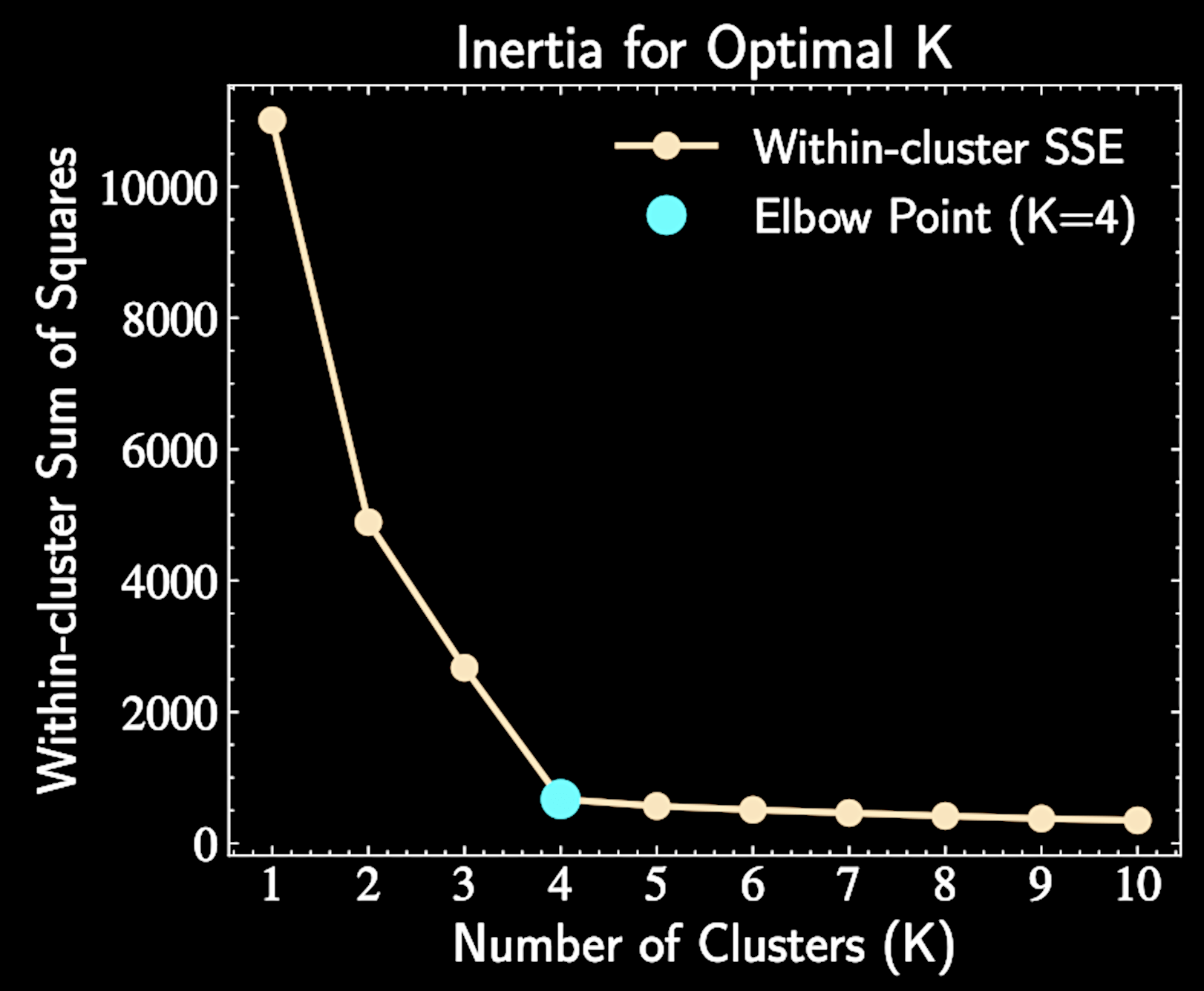
Determining the Number of Clusters
All clustering techniques discussed assume a fixed number of clusters K, which must be specified in advance
Determining the appropriate K value is a challenge
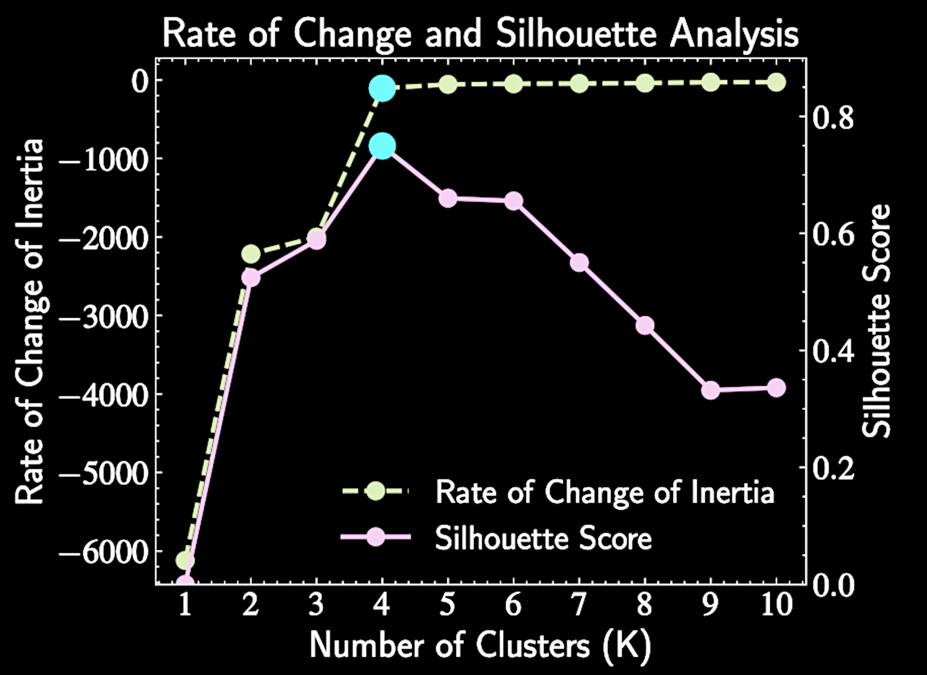
Methods like calculating the Initial and performance Silhouette Analysis provide quantitative guidance
Information Criterion (toward the end) is another theoeretical option
Inertial
Within-cluster sum of squares against increasing values of K (number of clusters)
The inertia is defined as:
With natural clusters \(K*\), adding clusters when \(K < K*\) reduces inertia, while \(K > K*\) yields diminishing returns
\text{SSE} = \sum_{k=1}^K \sum_{n \in C_k} |\mathbf{x}_n - \boldsymbol{\mu}_k|^2
Silhouette Analysis
For each point i, the score is:
\( a(i) = \) average distance between point i and all other points in the same cluster, \( b(i) = \) minimum average distance between point i and points in any other cluster
The optimal K maximizes the average silhouette score across all data points.
s(i) = \frac{b(i) - a(i)}{\max{(a(i), b(i))}}
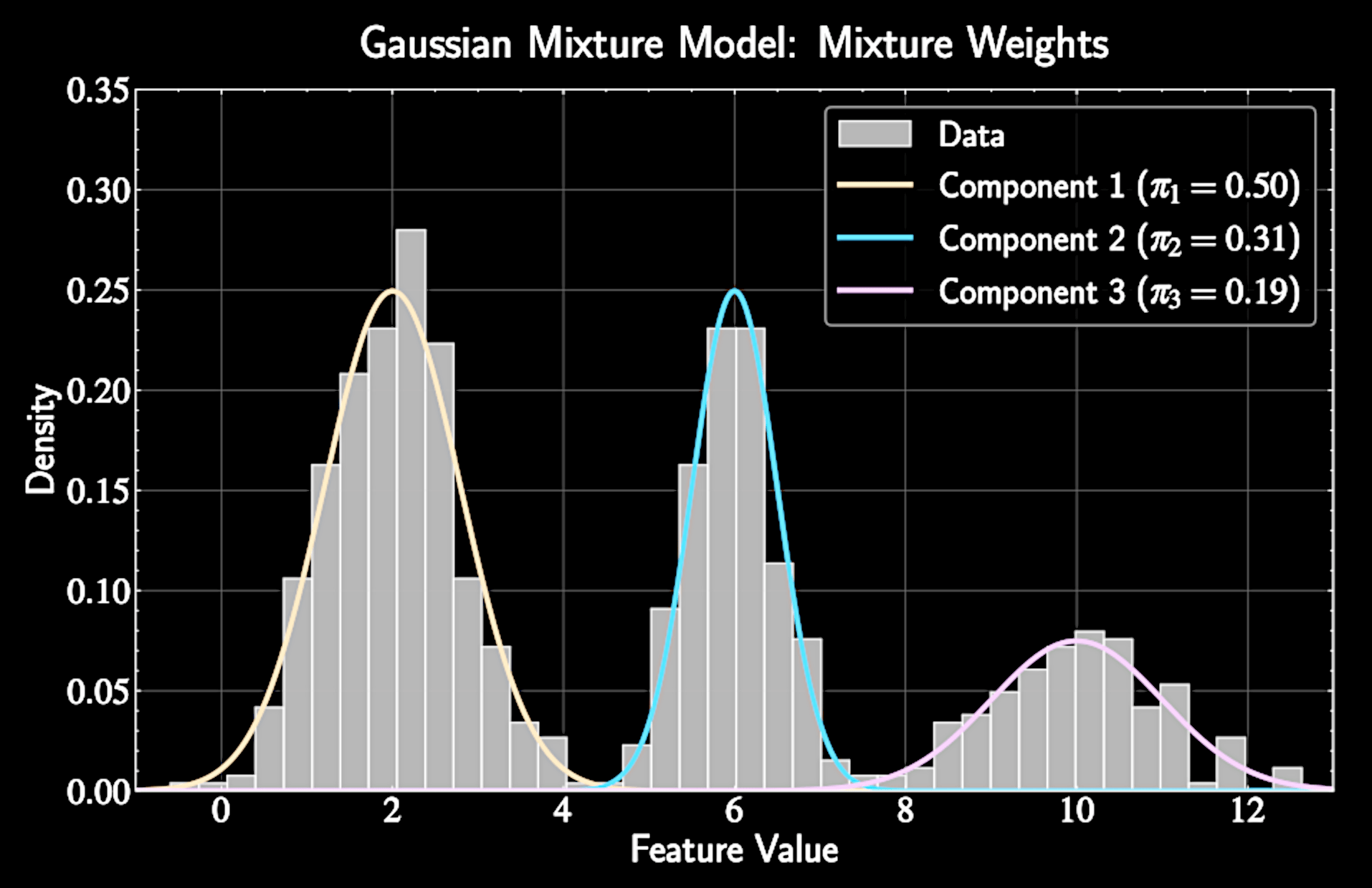
Gaussian Mixture Models
Data is modeled as generated from a weighted sum of multiple Gaussian distributions
p(\mathbf{x}) = \sum_{k=1}^K \pi_k \mathcal{N}(\mathbf{x}|\boldsymbol{\mu}_k, \boldsymbol{\Sigma}_k)
\(\pi_k\): Mixture weight representing prior probability of cluster k
Constraints: \(\pi_k \geq 0\) for all k and \(\sum_{k=1}^K \pi_k = 1\)
GMM Parameters to Optimize
Total free parameters: \((K-1) + KD + KD(D+1)/2\) (grows quadratically with dimension D)
\(\pi_k\): Relative importance of each component : \( K - 1 \) dimensions
Mean vectors \(\boldsymbol{\mu}_k\): \( K D \) dimensions
Covariance matrices \(\boldsymbol{\Sigma}_k\): \( K D (D+1)/2 \) dimensions
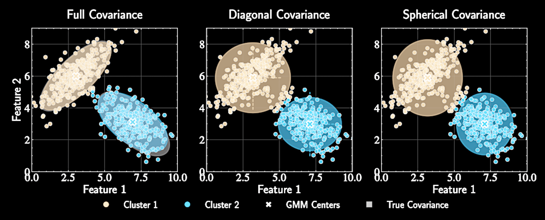
Simplifying Covariance Structures
Full covariance matrices: \(\boldsymbol{\Sigma}_k\) with \(K \cdot D(D+1)/2\) parameters
Diagonal covariance: \(\boldsymbol{\Sigma}_k = \text{diag}(\sigma_{k1}^2, \sigma_{k2}^2, \ldots, \sigma_{kD}^2)\) with \(K \cdot D\) parameters
Spherical covariance: \(\boldsymbol{\Sigma}_k = \sigma_k^2\mathbf{I}\) with just \(K\) parameters - K-means with soft assignments
Trade-off between model flexibility and computational efficiency
Logistics
Homework Assignment 4 due next Friday,11:59pm
Group Project 2 - Project Selection - feedback found on Carmen
Group Project 2 - Presentation - April 18
Group Project 2 - Report - April 28 (no deferment)
GMM Likelihood Function
Likelihood function:
Log-likelihood:
p(\{\mathbf{x}_n\}|\{\pi_k\}, \{\boldsymbol{\mu}_k\}, \{\boldsymbol{\Sigma}_k\}) = \prod_{n=1}^N \left[\sum_{k=1}^K \pi_k \mathcal{N}(\mathbf{x}_n|\boldsymbol{\mu}_k, \boldsymbol{\Sigma}_k)\right]
\ln p(\{\mathbf{x}_n\}|\{\pi_k\}, \{\boldsymbol{\mu}_k\}, \{\boldsymbol{\Sigma}_k\}) = \sum_{n=1}^N \ln\left[\sum_{k=1}^K \pi_k \mathcal{N}(\mathbf{x}_n|\boldsymbol{\mu}_k, \boldsymbol{\Sigma}_k)\right]
Challenges in GMM Optimization
Highly multimodal likelihood surface with many local maxima
Interdependence of parameters: optimal values of means depend on covariances and weights
Label switching problem: \( K! \) equivalent modes due to component index permutation
Need a specialized approach to decompose this complex problem into simpler ones
The EM Algorithm for GMMs
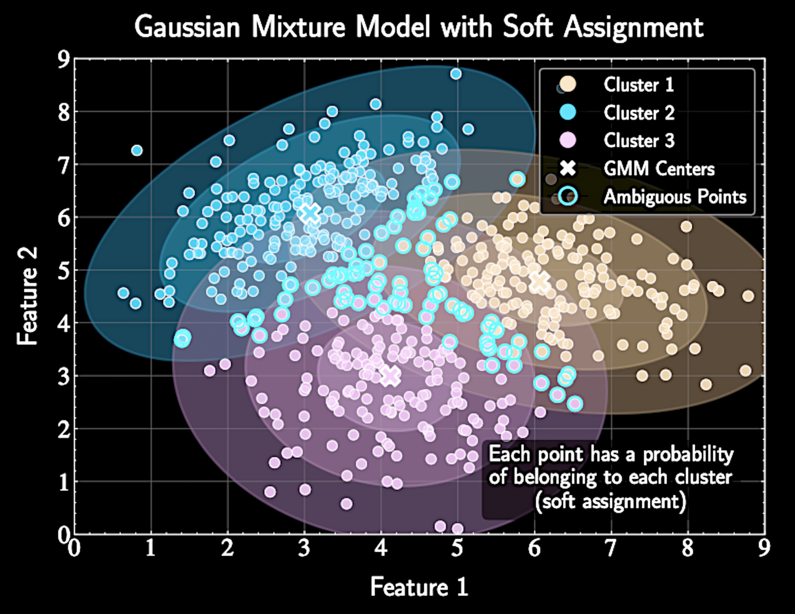
Introduces latent variables to overcome optimization challenges
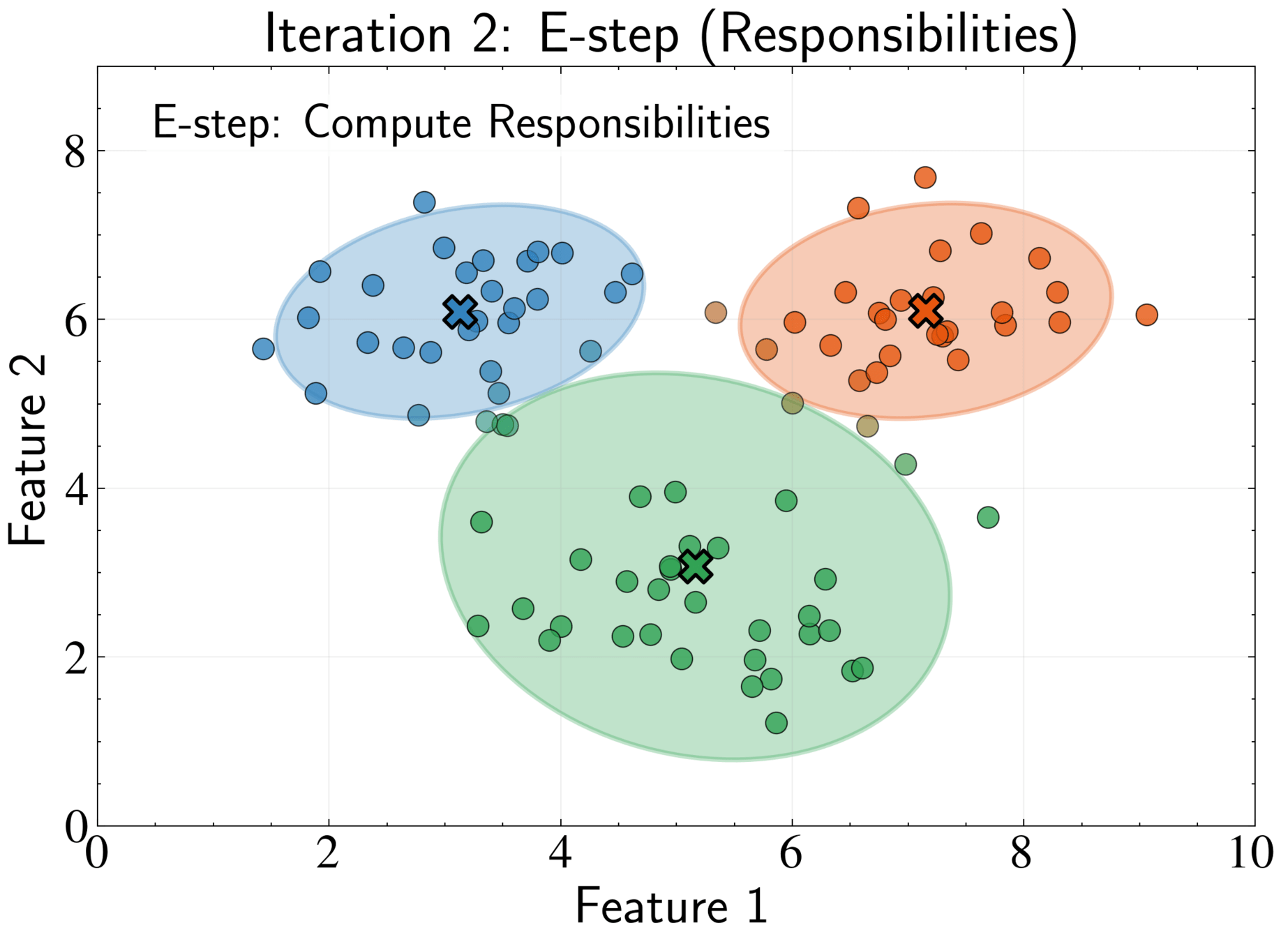
Responsibility \(\gamma_{nk}\) represents posterior probability that component k generated point n
Soft assignment allows partial membership in multiple clusters
\gamma_{nk} = \frac{\pi_k \mathcal{N}(\mathbf{x}_n|\boldsymbol{\mu}_k, \boldsymbol{\Sigma}_k)}{\sum_{j=1}^K \pi_j \mathcal{N}(\mathbf{x}_n|\boldsymbol{\mu}_j, \boldsymbol{\Sigma}_j)}

Deriving the Log-Likelihood Gradient
Start with log-likelihood:
Take derivative with respect to \(\boldsymbol{\mu}_k\):
\ln p(\{\mathbf{x}_n\}) = \sum_{n=1}^N \ln\left[\sum_{k=1}^K \pi_k \mathcal{N}(\mathbf{x}_n|\boldsymbol{\mu}_k, \boldsymbol{\Sigma}_k)\right]
\frac{\partial}{\partial \boldsymbol{\mu}_k} \ln p = \sum_{n=1}^N \frac{\partial}{\partial \boldsymbol{\mu}_k} \ln\left[\sum_{j=1}^K \pi_j \mathcal{N}(\mathbf{x}_n|\boldsymbol{\mu}_j, \boldsymbol{\Sigma}_j)\right]
Deriving the Log-Likelihood Gradient
Only term with \(\boldsymbol{\mu}_k\) survives in summation:
\frac{\partial}{\partial \boldsymbol{\mu}_k} \ln p = \sum_{n=1}^N \frac{1}{\sum_{j=1}^K \pi_j \mathcal{N}(\mathbf{x}_n|\boldsymbol{\mu}_j, \boldsymbol{\Sigma}_j)} \cdot \frac{\partial}{\partial \boldsymbol{\mu}_k}\left[\pi_k \mathcal{N}(\mathbf{x}_n|\boldsymbol{\mu}_k, \boldsymbol{\Sigma}_k)\right]
Deriving the Log-Likelihood Gradient
Derivating the Gaussian
Substitute back into our expression:
\frac{\partial}{\partial \boldsymbol{\mu}_k}\mathcal{N}(\mathbf{x}_n|\boldsymbol{\mu}_k, \boldsymbol{\Sigma}_k) = \mathcal{N}(\mathbf{x}_n|\boldsymbol{\mu}_k, \boldsymbol{\Sigma}_k) \cdot \boldsymbol{\Sigma}_k^{-1}(\mathbf{x}_n - \boldsymbol{\mu}_k)
\frac{\partial}{\partial \boldsymbol{\mu}_k} \ln p = \sum_{n=1}^N \frac{\pi_k \mathcal{N}(\mathbf{x}_n|\boldsymbol{\mu}_k, \boldsymbol{\Sigma}_k)}{\sum_{j=1}^K \pi_j \mathcal{N}(\mathbf{x}_n|\boldsymbol{\mu}_j, \boldsymbol{\Sigma}_j)} \cdot \boldsymbol{\Sigma}_k^{-1}(\mathbf{x}_n - \boldsymbol{\mu}_k)
Simplifying the Likelihood Gradient
Substituting responsibilities:
Responsibilities are treated as fixed during the M-step
\frac{\partial}{\partial \boldsymbol{\mu}_k} \ln p = \sum_{n=1}^N \gamma_{nk} \cdot \boldsymbol{\Sigma}_k^{-1}(\mathbf{x}_n - \boldsymbol{\mu}_k)
Deriving the Mean Update
Set derivative equal to zero and solve:
\sum_{n=1}^N \gamma_{nk} \cdot \boldsymbol{\Sigma}_k^{-1}(\mathbf{x}_n - \boldsymbol{\mu}_k) = 0
\Rightarrow \boldsymbol{\mu}_k = \frac{\sum_{n=1}^N \gamma_{nk} \cdot \mathbf{x}_n}{\sum_{n=1}^N \gamma_{nk}}
Define effective number of points in cluster k: \(N_k = \sum_{n=1}^N \gamma_{nk}\)
\boldsymbol{\mu}_k = \frac{1}{N_k}\sum_{n=1}^N \gamma_{nk}\mathbf{x}_n
Deriving the Mean Update
Compare with K-means update:
\boldsymbol{\mu}_k = \frac{\sum_{n=1}^N r_{nk} \cdot \mathbf{x}_n}{\sum_{n=1}^N r_{nk}}
GMMs generalize K-means by replacing hard assignments with soft responsibilities
\boldsymbol{\mu}_k = \frac{1}{N_k}\sum_{n=1}^N \gamma_{nk}\mathbf{x}_n
Deriving the Covariance Matrix Update
Start with multivariate Gaussian distribution:
\ln \mathcal{N}(\mathbf{x}|\boldsymbol{\mu}, \boldsymbol{\Sigma}) = -\frac{D}{2}\ln(2\pi) - \frac{1}{2}\ln|\boldsymbol{\Sigma}| - \frac{1}{2}(\mathbf{x} - \boldsymbol{\mu})^T\boldsymbol{\Sigma}^{-1}(\mathbf{x} - \boldsymbol{\mu})
We will differentiate with respect to precision matrix \(\boldsymbol{\Sigma}_k^{-1}\) instead of \(\boldsymbol{\Sigma}_k\)
Matrix calculus
\frac{\partial}{\partial \mathbf{A}} \ln|\mathbf{A}| = \mathbf{A}^{-1}
Differentiating the Log-Likelihood
Start with log-likelihood derivative:
\frac{\partial \ln p}{\partial \boldsymbol{\Sigma}_k^{-1}} = \sum_{n=1}^N \frac{1}{\sum_{j=1}^K \pi_j \mathcal{N}(\mathbf{x}_n|\boldsymbol{\mu}_j, \boldsymbol{\Sigma}_j)} \cdot \frac{\partial}{\partial \boldsymbol{\Sigma}_k^{-1}}\left[\pi_k \mathcal{N}(\mathbf{x}_n|\boldsymbol{\mu}_k, \boldsymbol{\Sigma}_k)\right]
Apply chain rule in form \(\frac{d}{dx}f(x) = f(x) \cdot \frac{d}{dx}\ln f(x)\):
\frac{\partial \ln p}{\partial \boldsymbol{\Sigma}_k^{-1}} = \sum_{n=1}^N \frac{\pi_k \mathcal{N}(\mathbf{x}_n|\boldsymbol{\mu}_k, \boldsymbol{\Sigma}_k)}{\sum_{j=1}^K \pi_j \mathcal{N}(\mathbf{x}_n|\boldsymbol{\mu}_j, \boldsymbol{\Sigma}_j)} \cdot \frac{\partial}{\partial \boldsymbol{\Sigma}_k^{-1}} \ln \mathcal{N}(\mathbf{x}_n|\boldsymbol{\mu}_k, \boldsymbol{\Sigma}_k)
Differentiating the Log-Likelihood
First term is the responsibility \(\gamma_{nk}\)
Need to calculate derivative of log Gaussian with respect to precision matrix \( \boldsymbol{\Sigma}_k^{-1} \)
\frac{\partial \ln p}{\partial \boldsymbol{\Sigma}_k^{-1}} = \sum_{n=1}^N \gamma_{nk} \frac{\partial}{\partial \boldsymbol{\Sigma}_k^{-1}} \ln \mathcal{N}(\mathbf{x}_n|\boldsymbol{\mu}_k, \boldsymbol{\Sigma}_k)
Derivative of Log Gaussian
Expand and rewrite terms involving \(\boldsymbol{\Sigma}_k\):
Apply matrix calculus identity \( \frac{\partial}{\partial \mathbf{A}} \ln|\mathbf{A}| = \mathbf{A}^{-1} \):
\frac{\partial}{\partial \boldsymbol{\Sigma}_k^{-1}} \left[-\frac{D}{2}\ln(2\pi) + \frac{1}{2}\ln|\boldsymbol{\Sigma}_k^{-1}| - \frac{1}{2}(\mathbf{x}_n - \boldsymbol{\mu}_k)^T\boldsymbol{\Sigma}_k^{-1}(\mathbf{x}_n - \boldsymbol{\mu}_k)\right]
\frac{\partial}{\partial \boldsymbol{\Sigma}_k^{-1}} \ln \mathcal{N}(\mathbf{x}_n|\boldsymbol{\mu}_k, \boldsymbol{\Sigma}_k) = \frac{1}{2}\boldsymbol{\Sigma}_k - \frac{1}{2}(\mathbf{x}_n - \boldsymbol{\mu}_k)(\mathbf{x}_n - \boldsymbol{\mu}_k)^T
Complete Log-Likelihood Derivative
Substitute derivative of log Gaussian back into log-likelihood and set equal to zero to find critical point:
Solve for \(\boldsymbol{\Sigma}_k\):
\sum_{n=1}^N \gamma_{nk} \left[\frac{1}{2}\boldsymbol{\Sigma}_k - \frac{1}{2}(\mathbf{x}_n - \boldsymbol{\mu}_k)(\mathbf{x}_n - \boldsymbol{\mu}_k)^T\right] = 0
\boldsymbol{\Sigma}_k = \frac{1}{N_k} \sum_{n=1}^N \gamma_{nk}(\mathbf{x}_n - \boldsymbol{\mu}_k)(\mathbf{x}_n - \boldsymbol{\mu}_k)^T
Interpreting the Covariance Update
Generalization of sample covariance matrix:
But with fractional point assignments through responsibilities \(\gamma_{nk}\)
\mathbf{S} = \frac{1}{N}\sum_{n=1}^N (\mathbf{x}_n - \boldsymbol{\mu})(\mathbf{x}_n - \boldsymbol{\mu})^T
\boldsymbol{\Sigma}_k = \frac{1}{N_k} \sum_{n=1}^N \gamma_{nk}(\mathbf{x}_n - \boldsymbol{\mu}_k)(\mathbf{x}_n - \boldsymbol{\mu}_k)^T
Optimizing Mixture Weights
Need to optimize mixture weights \(\pi_k\) while respecting constraint \(\sum_{k=1}^K \pi_k = 1\)
Use Lagrange multipliers for constrained optimization
First term is log-likelihood, second term enforces constraint via multiplier \(\lambda\)
\mathcal{L} = \ln p(\{\mathbf{x}_n\}) + \lambda\left(1 - \sum_{k=1}^K \pi_k\right)
Deriving the Update Equation
Take derivative with respect to \(\pi_k\) and set to zero:
Need to determine value of Lagrange multiplier \(\lambda\)
\frac{\partial \mathcal{L}}{\partial \pi_k} = \frac{\partial}{\partial \pi_k}\sum_{n=1}^N \ln\left[\sum_{j=1}^K \pi_j \mathcal{N}(\mathbf{x}_n|\boldsymbol{\mu}_j, \boldsymbol{\Sigma}_j)\right] - \lambda
= \sum_{n=1}^N \frac{1}{\sum_{j=1}^K \pi_j \mathcal{N}(\mathbf{x}_n|\boldsymbol{\mu}_j, \boldsymbol{\Sigma}_j)} \cdot \mathcal{N}(\mathbf{x}_n|\boldsymbol{\mu}_k, \boldsymbol{\Sigma}_k) - \lambda = 0
Finding the Lagrange Multiplier
Multiply both sides by \(\pi_k\), Sum both sides over all k, using constraint \(\sum_{k=1}^K \pi_k = 1\):
Inner numerator sum equals denominator, so fraction equals 1 for each point
\sum_{k=1}^K \pi_k \sum_{n=1}^N \frac{\mathcal{N}(\mathbf{x}_n|\boldsymbol{\mu}_k, \boldsymbol{\Sigma}_k)}{\sum_{j=1}^K \pi_j \mathcal{N}(\mathbf{x}_n|\boldsymbol{\mu}_j, \boldsymbol{\Sigma}_j)} - \lambda = 0
\lambda = N
Final Update Equation for Weights
Substitute \(\lambda = N\) back into our equation:
Recognize that the fraction is the responsibility \(\gamma_{nk}\):
\sum_{n=1}^N \frac{\pi_k \mathcal{N}(\mathbf{x}_n|\boldsymbol{\mu}_k, \boldsymbol{\Sigma}_k)}{\sum_{j=1}^K \pi_j \mathcal{N}(\mathbf{x}_n|\boldsymbol{\mu}_j, \boldsymbol{\Sigma}_j)} = N \pi_k
\pi_k = \frac{1}{N}\sum_{n=1}^N \gamma_{nk} = \frac{N_k}{N}
Proportion of data effectively "owned" by component k
Completing the EM Algorithm
So far: derived update equations for \(\boldsymbol{\mu}_k\), \(\boldsymbol{\Sigma}_k\), and \(\pi_k\) (M-step)
Alternate with computing optimal responsibilities (E-step)
\gamma_{nk} = \frac{\pi_k \mathcal{N}(\mathbf{x}_n|\boldsymbol{\mu}_k, \boldsymbol{\Sigma}_k)}{\sum_{j=1}^K \pi_j \mathcal{N}(\mathbf{x}_n|\boldsymbol{\mu}_j, \boldsymbol{\Sigma}_j)}
When model parameters are fixed, responsibilities are given by
Completing the EM Algorithm
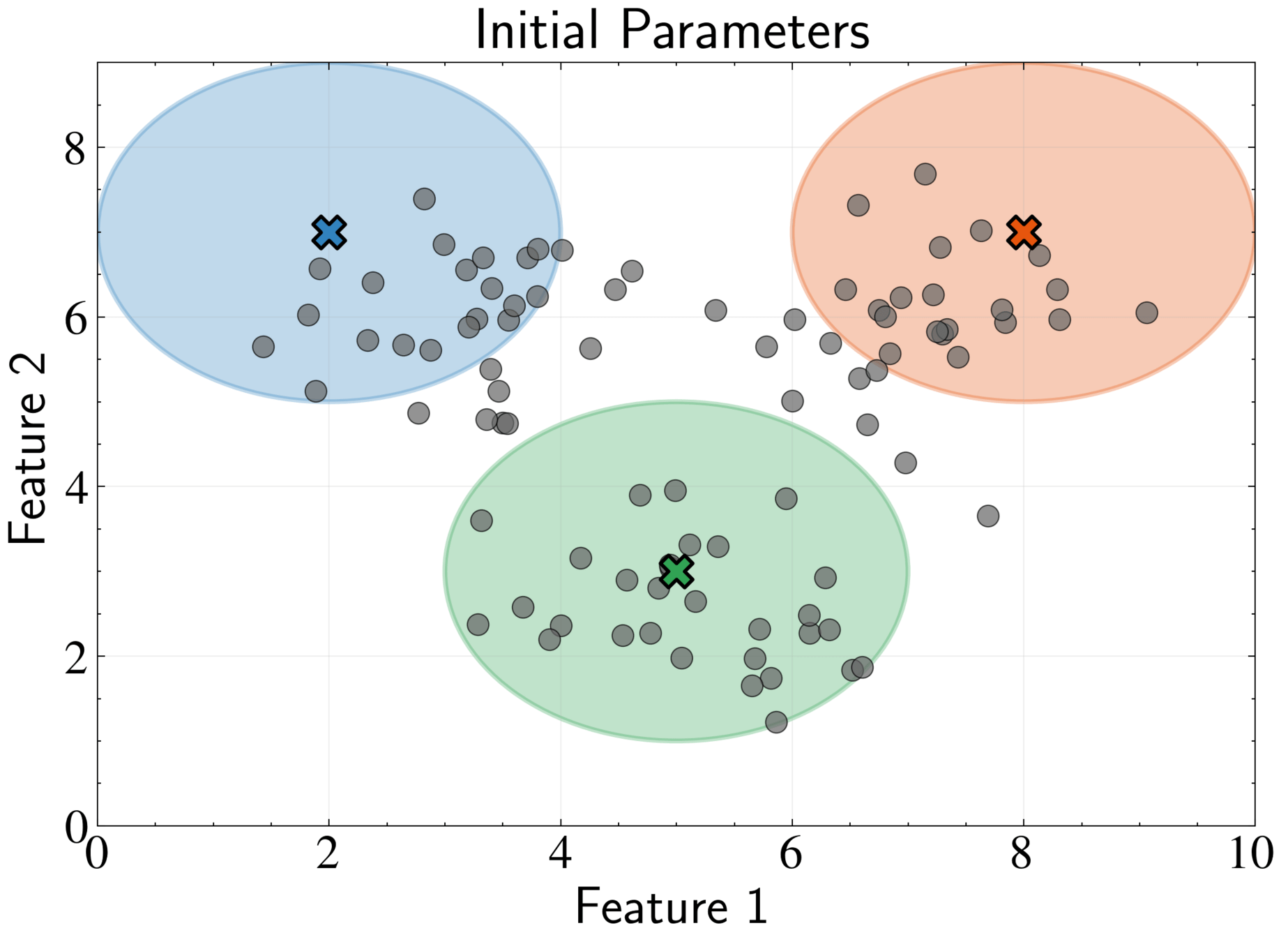
Initialization: Choose starting values for \({\pi_k}, {\boldsymbol{\mu}_k}, {\boldsymbol{\Sigma}_k}\)
Options:
- random data points as means,
- K-means results,
- random partitioning
Typically initialize weights uniformly: \(\pi_k = 1/K\)
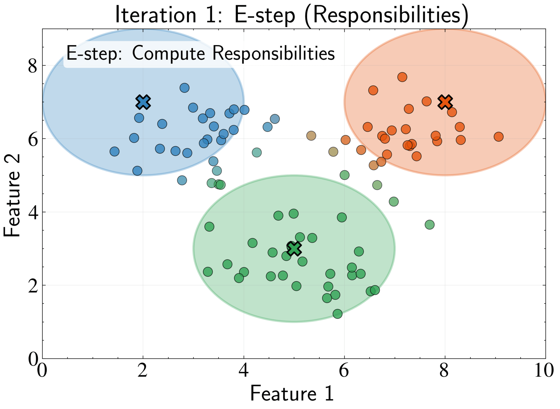
Completing the EM Algorithm
E-step: Compute responsibilities using current parameters
\gamma_{nk} = \frac{\pi_k \mathcal{N}(\mathbf{x}_n|\boldsymbol{\mu}_k, \boldsymbol{\Sigma}_k)}{\sum_{j=1}^K \pi_j \mathcal{N}(\mathbf{x}_n|\boldsymbol{\mu}_j, \boldsymbol{\Sigma}_j)}
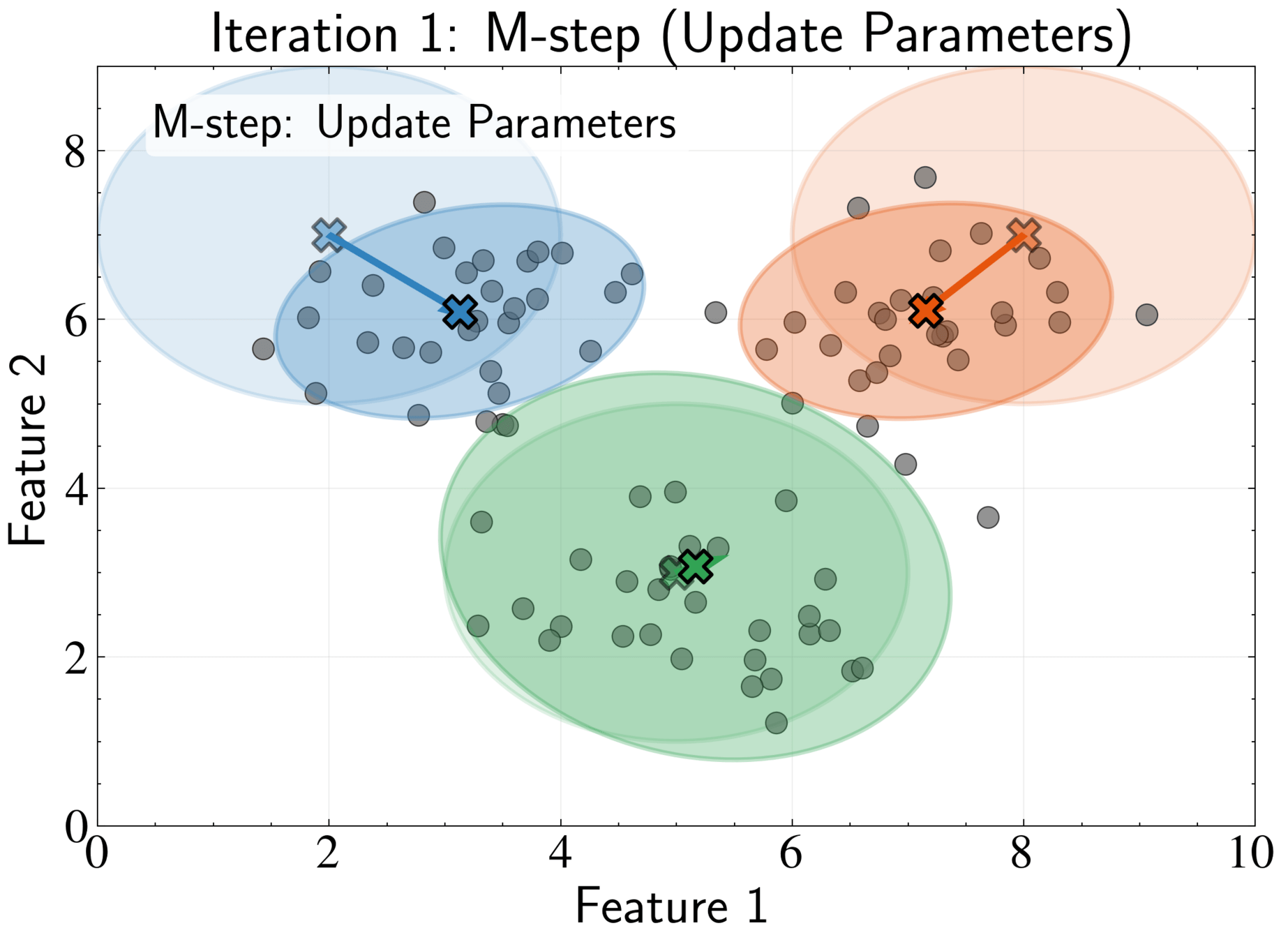
Completing the EM Algorithm
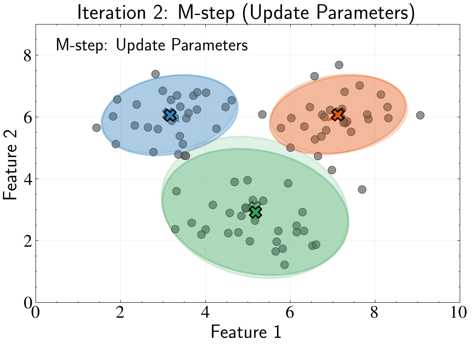
M-step: Update parameters using current responsibilities
N_k = \sum_{n=1}^N \gamma_{nk}
\boldsymbol{\mu}_k^{new} = \frac{1}{N_k}\sum_{n=1}^N \gamma_{nk}\mathbf{x}_n
\boldsymbol{\Sigma}_k^{new} = \frac{1}{N_k}\sum_{n=1}^N \gamma_{nk}(\mathbf{x}_n - \boldsymbol{\mu}_k^{new})(\mathbf{x}_n - \boldsymbol{\mu}_k^{new})^T
Completing the EM Algorithm
M-step: Update parameters using current responsibilities
\pi_k^{new} = \frac{N_k}{N}
Check log-likelihood change; stop if below threshold or maximum iterations reached
Common practice: run algorithm multiple times with different initializations. Select solution with highest likelihood
Connection to K-means and Key Advantages
K-means is a special case of GMM with three constraints.
GMMs use soft assignments \((\gamma_{nk})\), providing natural measure of uncertainty.
GMMs model clusters with arbitrary elliptical shapes through covariance matrices
GMMs are generative models that capture full probability distribution of data
Probabilistic Foundation and Applications
Select component \(k\) with probability \(\pi_k\)
Sample from Gaussian \(\mathcal{N}(\boldsymbol{\mu}_k, \boldsymbol{\Sigma}_k)\)
Valuable for mock catalogs, testing survey selection functions, and forward modeling
Generative capabilities allow creation of synthetic data:
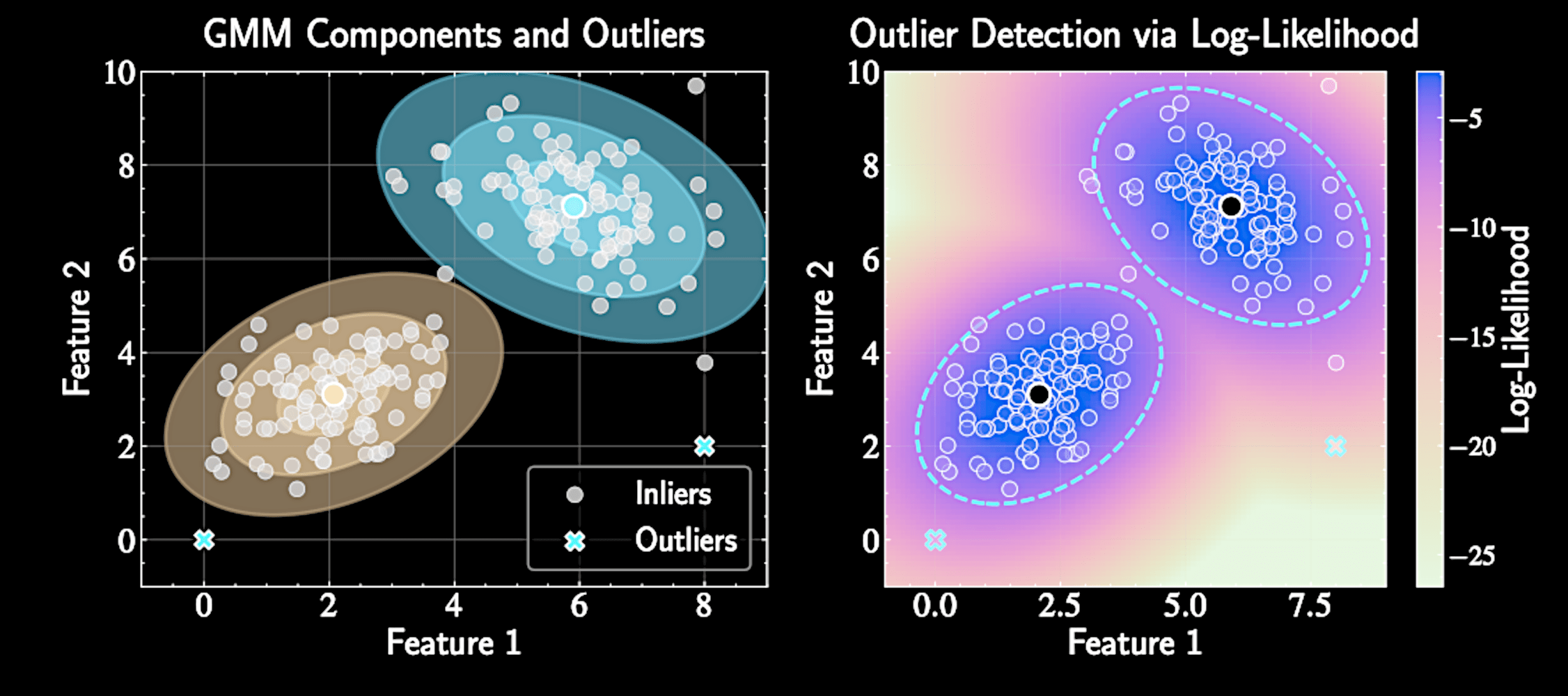
Outlier Detection
Low-density points identify potentially interesting astronomical objects
p(\mathbf{x}_*) = \sum_{k=1}^K \pi_k \mathcal{N}(\mathbf{x}_*|\boldsymbol{\mu}_k, \boldsymbol{\Sigma}_k) \ll 1
Enables principled outlier detection using probability density:
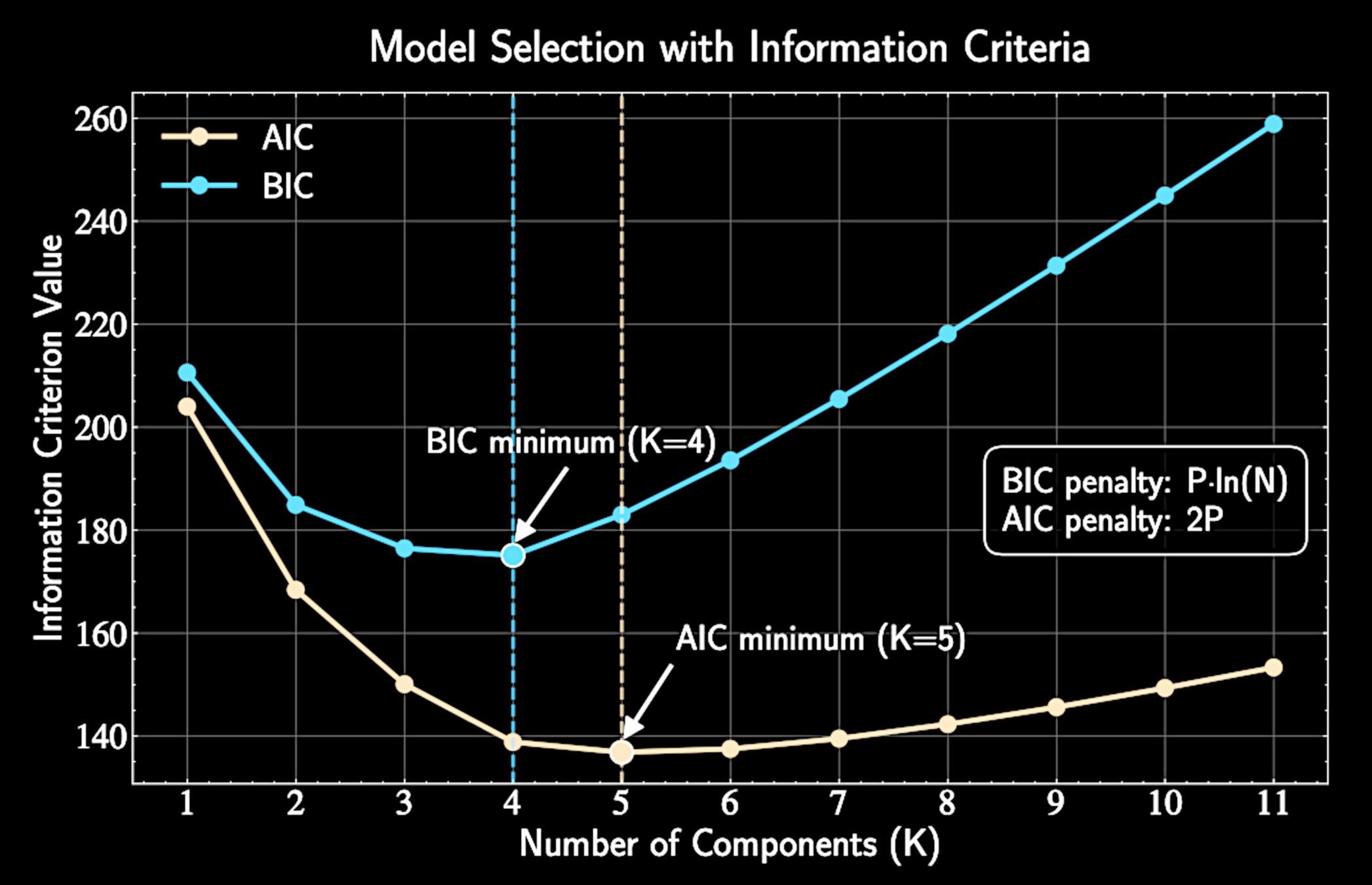
Model Selection with Information Criteria
As \(K\) increases, model complexity and data fit improve, with log-likelihood monotonically increasing
Extreme case: \(K=N\) gives perfect fit but learns nothing
Information criteria quantify the trade-off between fit and complexity
Determining the number of clusters \(K\)
Parsimony Principle
Occam's razor: When multiple models explain data equally well, prefer the simplest
Einstein: "Everything should be made as simple as possible, but no simpler"
Like regularization in regression, we penalize excessive
model complexity
Information-theoretic criteria provide principled statistical foundations for selection
Bayesian Information Criterion (BIC)
Information score (lower better):
\(\hat{L}\) is maximum likelihood, \( P \) is parameter count, \( N\) is data point count
BIC approximates the Bayes factor, comparing posterior probabilities of different models
\text{BIC} = -2\ln(\hat{L}) + P\ln(N)
Bayesian Information Criterion (BIC)
For a full-covariance GMM with \(K\) components in \(D\) dimensions:
P = (K-1) + KD + K\frac{D(D+1)}{2}
Bayesian Model Selection Framework
For model selection, compare the "evidence" of different models \(\mathcal{M}_K\):
p(\mathbf{X}|\mathcal{M}_K) = \int p(\mathbf{X}|\boldsymbol{\theta}_K, \mathcal{M}_K)p(\boldsymbol{\theta}_K|\mathcal{M}_K)d\boldsymbol{\theta}_K
Bayesian approach:
p(\boldsymbol{\theta}|\mathbf{X}) = \frac{p(\mathbf{X}|\boldsymbol{\theta})p(\boldsymbol{\theta})}{p(\mathbf{X})}
= \frac{p(\mathbf{X}|\boldsymbol{\theta},\mathcal{M}_K)p(\boldsymbol{\theta},\mathcal{M}_K)}{p(\mathbf{X}|\mathcal{M}_K)}
Laplace Approximation for BIC
Hessian
For intractable integrals, approximate log-posterior around its maximum:
\ln[p(\mathbf{X}|\boldsymbol{\theta}_K)p(\boldsymbol{\theta}_K)] \approx \ln[p(\mathbf{X}|\hat{\boldsymbol{\theta}}_K)p(\hat{\boldsymbol{\theta}}_K)]
- \frac{1}{2}(\boldsymbol{\theta}_K - \hat{\boldsymbol{\theta}}_K)^T \mathbf{H} (\boldsymbol{\theta}_K - \hat{\boldsymbol{\theta}}_K)
\mathbf{H} = -\nabla^2 \ln p(\mathbf{X}|\boldsymbol{\theta}_K) = -\sum_{n=1}^N \nabla^2 \ln p(\mathbf{x}_n|\boldsymbol{\theta}_K)
This gives \(\mathbf{H} = N \cdot \mathcal{J}(\hat{\boldsymbol{\theta}}_K)\) where \(\mathcal{J}\) is average information per observation
BIC Derivation and Asymptotic Behavior
The \((2\pi)^{P/2}|\mathbf{H}|^{-1/2}\) term is the normalization constant from the \(P\)-dimensional Gaussian Integrating:
Determinant property, for \(P\) parameters:
|\mathbf{H}| = |N \cdot \mathcal{J}(\hat{\boldsymbol{\theta}}_K)| = N^P \cdot |\mathcal{J}(\hat{\boldsymbol{\theta}}_K)|
p(\mathbf{X}|\mathcal{M}_K) \approx p(\mathbf{X}|\hat{\boldsymbol{\theta}}_K)p(\hat{\boldsymbol{\theta}}_K) \cdot (2\pi)^{P/2}|\mathbf{H}|^{-1/2}
This integration automatically implements Occam's razor by penalizing complex parameter spaces
Asymptotic Behavior and Final BIC Form
As \(N\) grows, log-likelihood \(\mathcal{O}(N)\) and penalty \(P\ln(N)\) dominate over \(\mathcal{O}(1)\) terms
Taking negative log:
2\ln p(\mathbf{X}|\mathcal{M}_K) \approx -2\ln p(\mathbf{X}|\hat{\boldsymbol{\theta}}_K) - 2\ln p(\hat{\boldsymbol{\theta}}_K) + P\ln(N) + \mathcal{O}(1)
This yields BIC:
\text{BIC} = -2\ln(\hat{L}) + P\ln(N)
Practical BIC Application for GMMs
Select model with lowest BIC value
Compute log-likelihood at EM convergence:
\ln(\hat{L}) = \sum_{n=1}^N \ln\left(\sum_{k=1}^K \hat{\pi}_k \mathcal{N}(\mathbf{x}_n|\hat{\boldsymbol{\mu}}_k, \hat{\boldsymbol{\Sigma}}_k)\right)
BIC validity depends on large samples, well-behaved likelihoods, and diffuse priors
Akaike Information Criterion (AIC)
Smaller penalty than BIC: \(2P\) instead of \(P\ln(N)\)
AIC approaches model selection from information theory perspective
\text{AIC} = -2\ln(\hat{L}) + 2P
AIC tends to favor more complex models.
Information-Theoretic Intuition for AIC
Aims to maximize information between model and true data-generating process
AIC connects to entropy and mutual information concepts
Using same data to fit and evaluate introduces bias, larger for complex models
This bias is asymptotically approximated by parameter count \(P\)
Small Sample Correction for AIC
Correction provides more aggressive penalty when observations are limited
For limited samples, corrected AIC (AICc) is preferred:
As \(N\) increases, AICc converges to standard AIC
\text{AIC}_c = \text{AIC} + \frac{2P(P+1)}{N-P-1}
BIC vs. AIC: Philosophical Differences
AIC aims to find the model that will make the best predictions on new data
BIC attempts to identify the "true" model
Both criteria provide guidance but require domain knowledge for interpretation
Final decisions should integrate statistical evidence with scientific insight
What We Have Learned:
K-means
Gaussian Mixture Models
Expectation-Maximization Algorithm
Information Criterion
Astron 5550 - Lecture 11
By Yuan-Sen Ting


