Lecture 12 : Sampling and Monte Carlo Methods
Assoc. Prof. Yuan-Sen Ting
Astron 5550 : Advanced Astronomical Data Analysis
Logistics
Homework Assignment 4 due this Friday,11:59pm
Group Project 2 - Presentation - April 16 (Next Week, Wed)
Group Project 2 - Report - April 28 (no deferment)
Remote lecture this Wednesday (link on Carmen)
Plan for Today :
Grid-Based Sampling
Inverse Cumulative Distribution Function
Rejection Sampling
Importance Sampling
Sampling and Monte Carlo Methods
We've covered supervised learning (regression, classification) and unsupervised learning (PCA, clustering)
All involve maximizing likelihood and deriving posterior distributions
Posterior distribution always has the form:
p(\boldsymbol{\theta}|\mathcal{D}) \propto p(\mathcal{D}|\boldsymbol{\theta}) \cdot p(\boldsymbol{\theta})
The Bayesian Framework
Knowing the mathematical form isn't enough for practical use
We need to draw samples or compute expectations
Many ML tasks require computing expectations:
E[f(z)] = \int f(z) p(z) dz
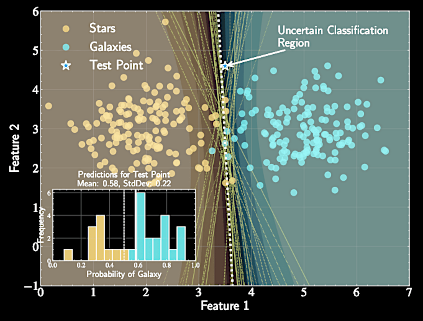
Posterior Predictive Distribution
Integrates over all parameter values weighted by posterior probability:
Allows us to make predictions for new observations
Accounts for all uncertainty in model parameters
p(y_*|x_*, \mathcal{D}) = \int p(y_*|x_*, \boldsymbol{\theta}) p(\boldsymbol{\theta}|\mathcal{D}) d\boldsymbol{\theta}
From Simple to Complex Model
Simple models (linear regression): Posterior is Gaussian, analytically tractable
Slightly non-linear models (logistic regression): Require approximations
Complex models (non-linear, hierarchical): Analytical solutions unavailable
Need methods to sample directly from complex posteriors
Monte Carlo Approximation
Approximate expectations using samples:
Samples \( z^{(1)}, z^{(2)}, \ldots, z^{(N)} \) drawn from distribution \( p(z) \)
Error decreases at rate of \( \mathcal{O}(1/\sqrt{N}) \) regardless of dimensionality
E[f(z)] = \int f(z) p(z) dz
E[f(z)] \approx \frac{1}{N} \sum_{l=1}^{N} f(z^{(l)})
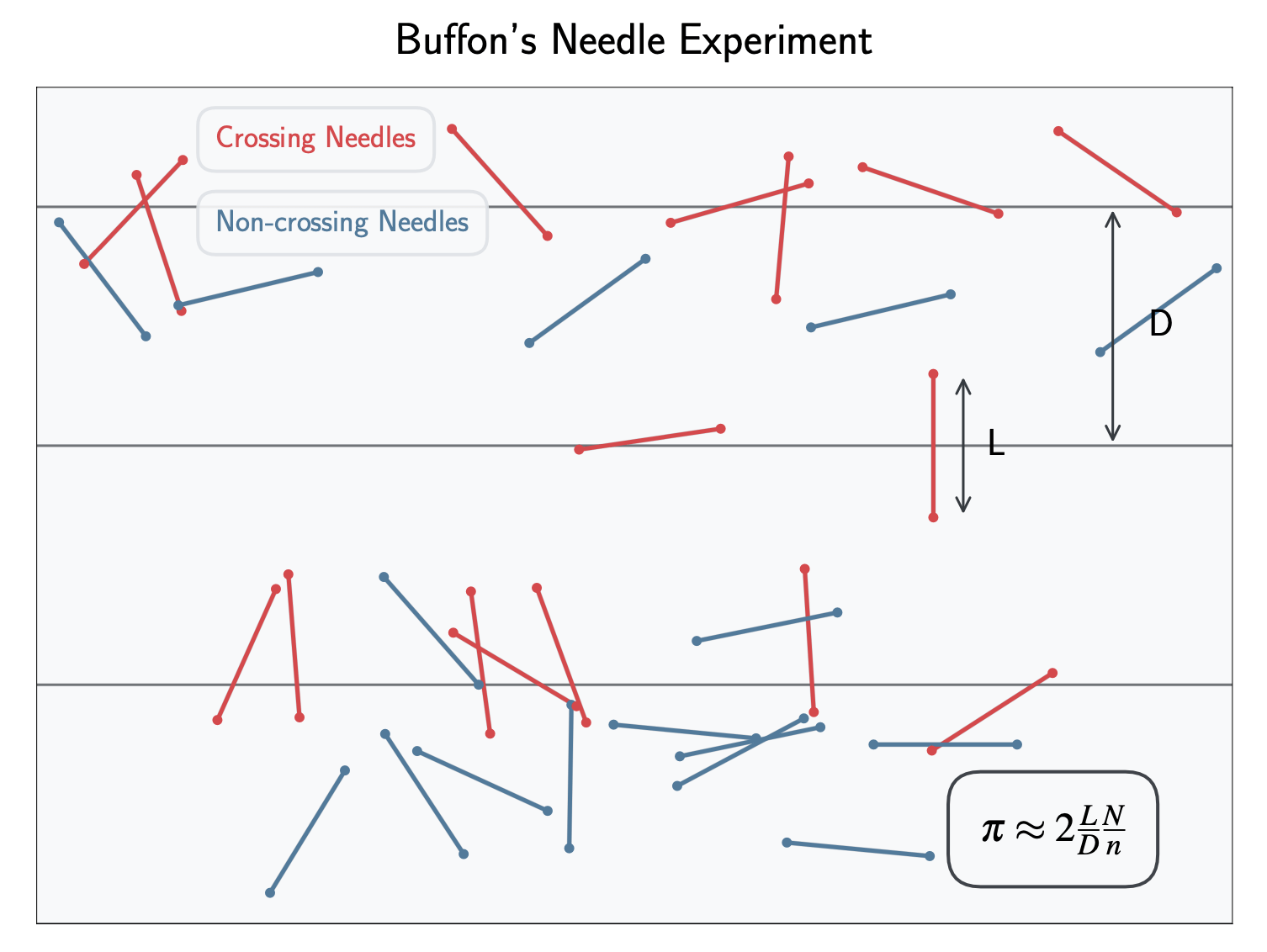
Buffon's Needle Experiment
Sampling has deep historical roots, predating modern computers
Buffon's needle experiment (18th century): A Monte Carlo method for estimating \( \pi \)
Drop needles of length \( L\) on floor with parallel lines spaced D apart \(L \leq D \)
p(\text{crossing}) = \int^\pi_0 \frac{L \sin \theta}{D \pi} d \theta
From Physical to Computational Randomization
Estimate \(\pi \) by:
Profound connection between physical randomization and numerical integration
Enables work with arbitrarily complex models while performing proper Bayesian inference
\pi \approx 2\frac{L}{D} \frac{N}{n}
N = total needles, n = crossing needles
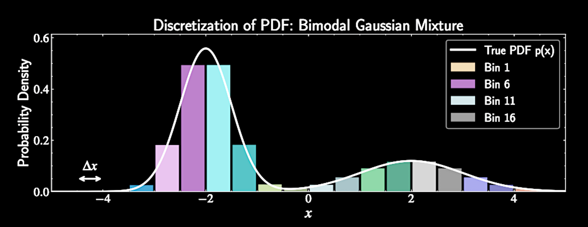
Grid-Based Sampling
Discretize continuous domain into equally spaced grid points
For domain \( [a,b] \):
Evaluate PDF at each grid point: \( p_i = p(x_i) \)
x_i = a + i\Delta x, \quad i = 0, 1, \ldots, n
Grid-Based Sampling
Discretize continuous domain into equally spaced grid points
For domain \( [a,b] \):
Evaluate PDF at each grid point: \( p_i = p(x_i) \)
x_i = a + i\Delta x, \quad i = 0, 1, \ldots, n
Normalized probabilities:
\tilde{p}_i = \frac{p_i}{Z} , \quad Z = \sum_{i=0}^{n} p_i
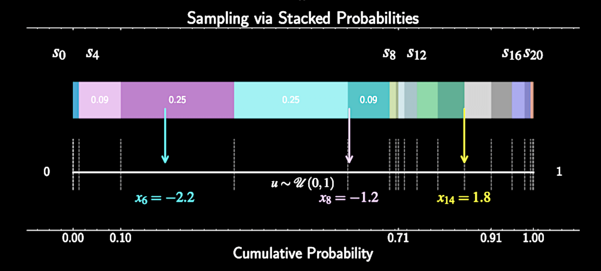
Generating Samples
Generate uniform random number \( u \sim \mathcal{U}(0, 1) \)
Compute partial sums: \( s_i = \sum_{j=0}^{i} \tilde{p}_j \) for \( i = 0, 1, \ldots, n \)
Find bin where \( s_{i-1} < u \leq s_i \)
Return corresponding grid point \( x_i \) as sample
Extension to Multiple Dimensions
For \(d\)-dimensional random variable, create \(d\)-dimensional grid
Grid points:
Evaluate joint PDF at each grid point and normalize
Sampling procedure similar to one-dimensional case, computing a flattened cumulative sum.
x_{i_1, i_2, \ldots, i_d} = (a_1 + i_1\Delta x_1, a_2 + i_2\Delta x_2, \ldots, a_d + i_d\Delta x_d)
Limitation of Grid-Based Sampling
Curse of dimensionality: Total bins scale as \( N^D \) exponential growth
Discretization error: Samples constrained to grid points
Only practical for low dimensions, e.g.,1D or 2D.
Inverse CDF Method: A Continuous Approach
Inverse CDF method: Limiting case of grid approach as bin width approaches zero
Works directly with continuous distributions rather than discretized approximations
Grid approach partial sums generalize to cumulative distribution function (CDF)
P(x) = \int_{-\infty}^{x} p(t) dt
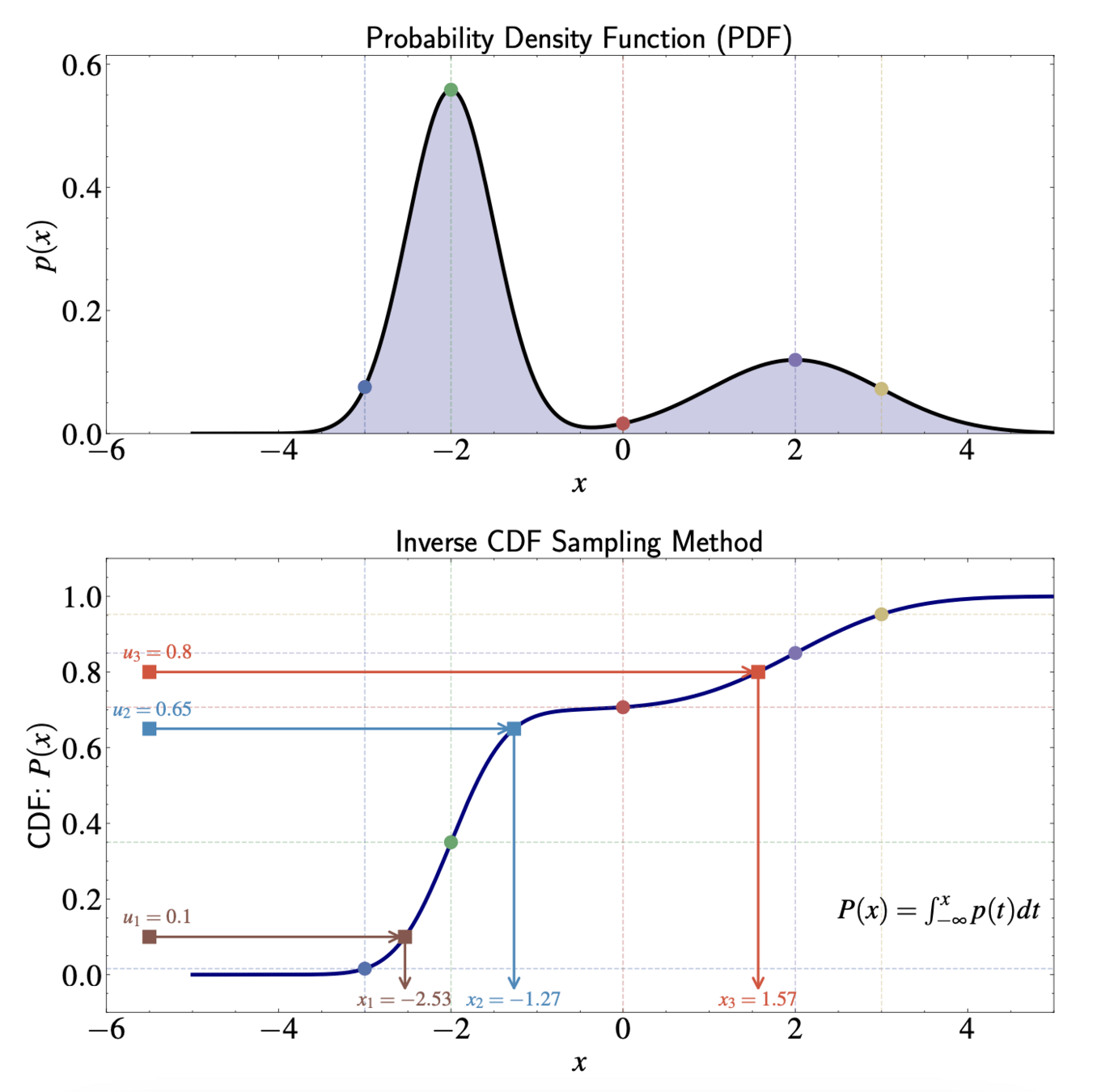
The Inverse CDF Method
Simple procedure for generating samples:
Generate uniform random number \( u \sim \mathcal{U}(0,1) \)
Compute \( x = P^{-1}(u) \), where \( P^{-1} \) is inverse of CDF
Return \( x \) as sample from target distribution
Geometric Interpretation
In regions of high PDF: CDF increases rapidly, samples compressed on x-axis
In regions of low PDF: CDF increases slowly, samples spread out on x-axis
Analytical Examples - Exponential Distribution
PDF: For \( x \geq 0 \)
CDF:
Inverse CDF:
Generating samples: Take negative logarithm of uniform random numbers, divide by \( \lambda \)
p(x) = \lambda e^{-\lambda x}
P(x) = 1 - e^{-\lambda x}
x = -\frac{1}{\lambda} \ln(1-u)
Analytical Examples - Power Law Distribution
PDF: \( p(x) = C x^{-\alpha} \) where \( \alpha > 1 \) and \( C = \frac{\alpha - 1}{x_{\min}^{1-\alpha} - x_{\max}^{1-\alpha}} \)
CDF:
Inverse CDF:
P(x) = \frac{x_{\min}^{1-\alpha} - x^{1-\alpha}}{x_{\min}^{1-\alpha} - x_{\max}^{1-\alpha}}
x = [x_{\min}^{1-\alpha} - u(x_{\min}^{1-\alpha} - x_{\max}^{1-\alpha})]^{\frac{1}{1-\alpha}}
Advantages of the Inverse CDF Method
Conceptually straightforward
Computationally efficient when inverse CDF can be calculated analytically
Generates samples that exactly follow target distribution
Limitations of the Inverse CDF Method
Requires closed-form expression for inverse CDF
Challenges with multivariate distributions
Rosenblatt transformation uses conditional distributions
Practical only when conditional distributions have known forms - rare cases
Rejection Sampling
More versatile than inverse CDF - handles distributions without closed-form inverse CDFs
Evaluating \( p(x) \) doesn't directly tell us how to generate samples
Transforms samples from simpler distribution to target distribution
Applicable to a broader class of distributions than previously discussed methods
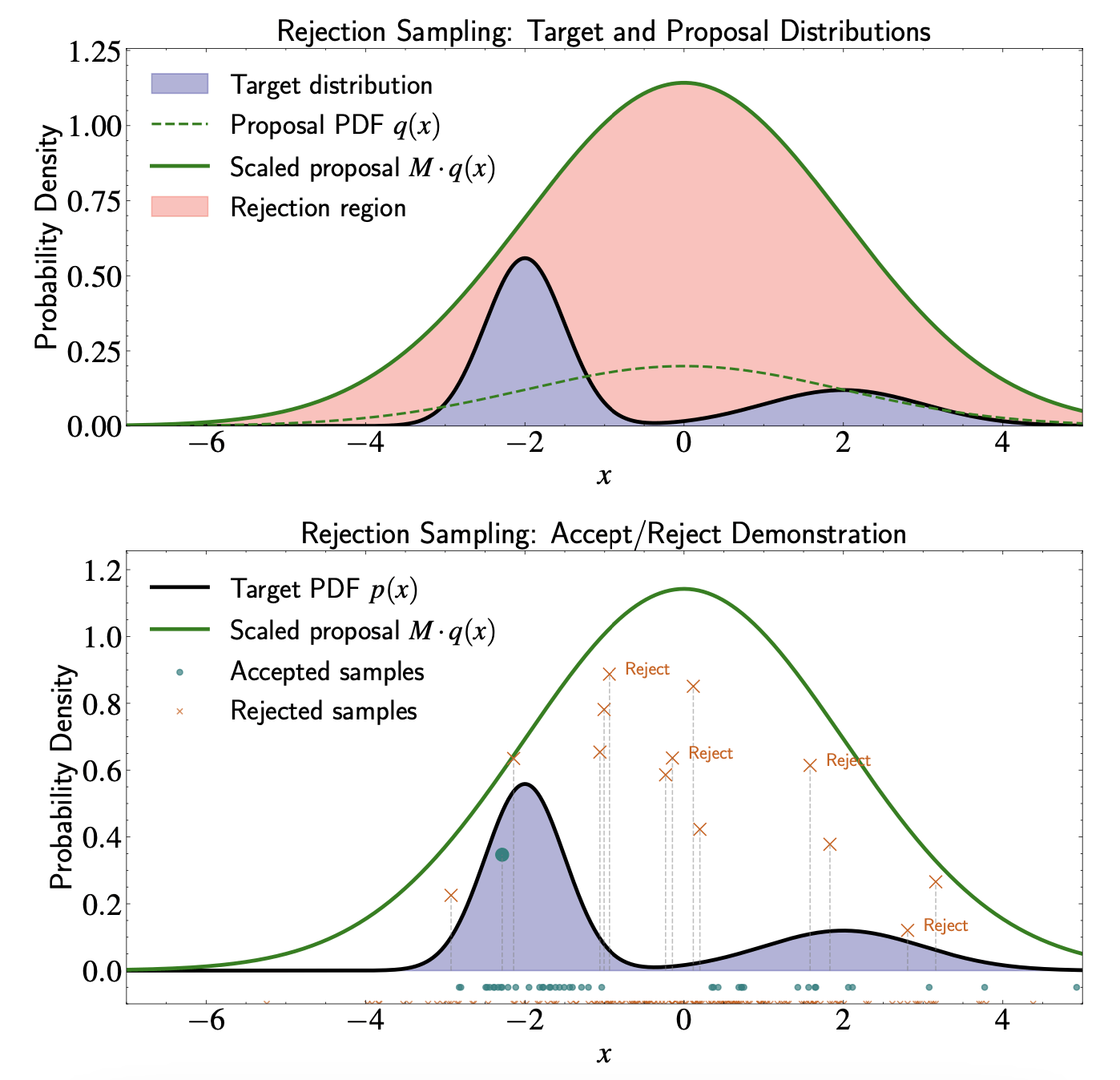
Proposal Distribution
Target distribution \( p(x) \) from which we want to draw samples
Proposal distribution: PDF \( q(x) \) that satisfies two requirements
Must be able to efficiently generate samples from \( q(x) \)
An envelope completely covering target distribution: Exists constant \( M \geq 1 \) such that \( M q(x) \geq p(x) \) for all \( x \)
Rejection Sampling Algorithm
Generate sample \( x_* \sim q(x) \) from proposal distribution
Compute acceptance ratio \( \)
Generate uniform random number \( u \sim \mathcal{U}(0, 1) \)
If \( u \leq \alpha \), accept \( x_* \) as sample from \( p(x) \); otherwise, reject
\alpha = \frac{p(x_*)}{M q(x_*)}
Efficiency Considerations
Optimal proposal distribution balances:
Ease of sampling from \( q(x) \)
Similarity to target \( p(x) \) in shape
Sufficient heavy tails to dominate \( p(x) \)
Advantages of Rejection Sampling
Extends naturally to multidimensional distribution
Works for any distribution we can evaluate
(even up to normalizing constant)
Requires minimal assumptions about target distribution
Limitations of Rejection Sampling
Efficiency deteriorates rapidly as dimensionality increases
Challenges with heavy-tailed distributions
Advanced techniques (MCMC) necessary for high-dimensional problems
Importance Sampling
Different approach from rejection sampling but shares some similarities
Efficiently estimating expectations rather than generating exact samples
Uses proposal distribution but weights samples instead of rejecting them
The Expectation Problem
Many problems involve computing expectations:
Direct Monte Carlo approach:
But we do not know how to sample from \( p(x) \)
E_{p}[f] = \int f(x) p(x) dx
E_{p}[f] \approx \frac{1}{N} \sum_{i=1}^{N} f(x^{(i)}),
x^{(i)} \sim p(x)
The Key Insight
Sample from proposal distribution \( q(x) \) that is easier to work with
E_{p}[f] = \int f(x) p(x) dx
= \int f(x) \frac{p(x)}{q(x)} q(x) dx
= E_{q}\left[f(x) \frac{p(x)}{q(x)}\right]
The Key Insight
This leads to importance sampling estimator:
E_{p}[f] \approx \frac{1}{N} \sum_{i=1}^{N} w(x^{(i)}) f(x^{(i)}),
w(x) = \frac{p(x)}{q(x)}
E_{q}\left[f(x) \frac{p(x)}{q(x)}\right]
x^{(i)} \sim q(x)
Importance weights defined as:
Handling Unnormalized Distributions
In Bayesian inference, we often know \( p(x) \) only up to normalizing constant:
p(x) = \frac{\tilde{p}(x)}{Z_p}
E_{p}[f] = \frac{1}{Z_p} \int f(x) \tilde{p}(x) dx = \frac{Z_q}{Z_p} \int f(x) \frac{\tilde{p}(x)}{\tilde{q}(x)} q(x) dx
Rewrite expectation:
Handling Unnormalized Distributions
Unnormalized importance weights:
\tilde{w}(x) = \frac{\tilde{p}(x)}{\tilde{q}(x)}
Z_p = \int \tilde{p}(x) dx = \int \frac{\tilde{p}(x)}{\tilde{q}(x)} \tilde{q}(x) dx
Normalization constant
= Z_q \int \frac{\tilde{p}(x)}{\tilde{q}(x)} q(x) dx = Z_q E_{q}\left[\frac{\tilde{p}(x)}{\tilde{q}(x)}\right]
Handling Unnormalized Distributions
Therefore:
\frac{Z_p}{Z_q} = E_q\left[\frac{\tilde{p}(x)}{\tilde{q}(x)}\right] \approx \frac{1}{N} \sum_{i=1}^{N} \tilde{w}(x^{(i)})
E_{p}[f] \approx \frac{\sum_{i=1}^{N} \tilde{w}(x^{(i)}) f(x^{(i)})}{\sum_{i=1}^{N} \tilde{w}(x^{(i)})},
Self-normalized estimator:
x^{(i)} \sim q(x)
Effective Sample Size
Finite sampling noise goes as \( 1 / \sqrt{\text{ESS}} \), instead of \( 1 / \sqrt{N} \)
Effective Sample Size (ESS):
Interpretation: Measures weight distribution evenness
Range: \( 1 \leq \text{ESS} \leq N \)
(equal weights → ESS = N, one dominant weight → ESS ≈ 1)
\text{ESS} \approx \frac{\left(\sum_{i=1}^{N} \tilde{w}(x^{(i)})\right)^2}{\sum_{i=1}^{N} \tilde{w}(x^{(i)})^2}
ESS and the Truncated Normal Example
Target: Standard normal truncated to region \( [5,\infty) \)
Standard normal: With \( N = 10^7 \) samples, expect only 3 non-zero weights. ESS = 3 regardless of the samples generated
Better proposal (shifted exponential):
\( q(x) = \lambda e^{-\lambda(x-5)} \cdot \mathbf{1}(x \geq 5) \)
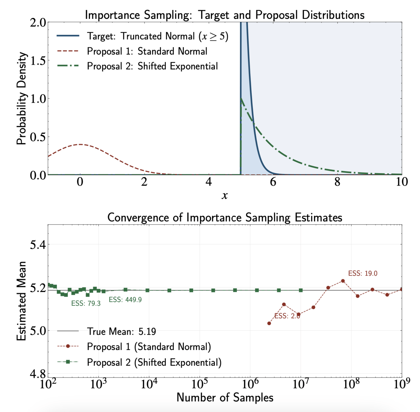
Proposal Distribution Selection Principles
Support coverage: \( q(x) > 0 \) whenever \( f(x)p(x) \neq 0 \)
Maximize effective sample size: Ideally \( q(x) \propto |f(x)|p(x) \)
Tail behavior: \( q(x) \) should have heavier tails than \( p(x) \)
Tractability: \( q(x) \) should be easy to sample from and evaluate
What We Have Learned:
Grid-Based Sampling
Inverse Cumulative Distribution Function
Rejection Sampling
Importance Sampling
Astron 5550 - Lecture 12
By Yuan-Sen Ting


