Lecture 9 : Bayesian Logistic Regression
Assoc. Prof. Yuan-Sen Ting
Astron 5550 : Advanced Astronomical Data Analysis
Logistics
Homework Assignment 3 due this Friday,11:59pm
Group Project Report due tonight, 11:59pm
Select and submit your topic for group project 2 (on Carmen), by next Friday, 11:59pm
I will be away next week. Lecture will be recorded and posted on Carmen
Plan for Today :
Bayesian Logistic Regression
Soft Boundary
Laplace Approximation
Probit Approximation
Logistic Regression Recap
Logistic regression uses linear weights \({w_k}\) to convert features into probabilities via logits
Maximum likelihood estimation optimizes weights using cross-entropy loss
Binary Logistic Regression Review
Binary classification uses sigmoid function to model class probability:
Likelihood function:
p(C_1|\mathbf{x}, \mathbf{w}) = \sigma(\mathbf{w}^T \mathbf{x}) = \frac{1}{1 + e^{-\mathbf{w}^T \mathbf{x}}}
p(\mathbf{t} | \mathbf{w}, \mathbf{X}) = \prod^N_{n=1} y_n^{t_n} (1 - y_n)^{(1-t_n)}
Astronomical Classification Challenges
Astronomical data suffers from scarcity of well-labeled examples
Training samples typically come from biased sampling (easier-to-classify objects)
Example: Galaxy classification datasets contain clear spiral/elliptical examples but few transitional morphologies
The Bayesian Perspective
Core insight: Model parameters \( \{ \mathbf{w} \} \) themselves have uncertainty
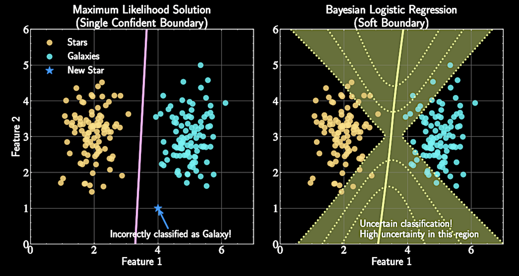
Multiple decision boundaries could reasonably separate classes given finite data
Rather than seeking single "best" model, characterize posterior distribution over all possible models
Bayesian Approach to Logistic Regression
Instead of single weight vector, we derive posterior distribution \(p(\mathbf{w}|\mathcal{D})\)
Provides naturally higher uncertainty in regions with sparse/no training data
Technical challenges: non-Gaussian posterior distribution requires approximation techniques (Laplace approximation, probit approximation)
Bayesian Framework for Logistic Regression
Start with prior distribution over weights:
Apply Bayes' theorem:
p(\mathbf{w}) = \mathcal{N}(\mathbf{w} | \mathbf{m}_0, \mathbf{S}_0)
p(\mathbf{w} | \mathbf{t}, \mathbf{X}) \propto p(\mathbf{w}) \cdot p(\mathbf{t} | \mathbf{w}, \mathbf{X})
The Non-Gaussian Posterior Challenge
Posterior distribution:
Unlike Bayesian linear regression, posterior is not Gaussian
No simple analytical form exists for this posterior distribution
p(\mathbf{w} | \mathbf{t}, \mathbf{X}) \propto \mathcal{N}(\mathbf{w} | \mathbf{m}_0, \mathbf{S}_0) \cdot \prod^N_{n=1} y_n^{t_n} (1 - y_n)^{(1-t_n)}
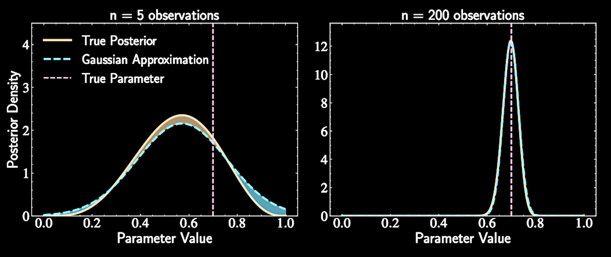
Bernstein-von Mises Theorem
Posteriors tend toward Gaussian distributions as sample size increases
Related to Central Limit Theorem
Each observation contributes information; aggregate effect produces increasingly Gaussian-shaped distribution
Solution preview: Laplace approximation will approximate this complex posterior with a Gaussian distribution
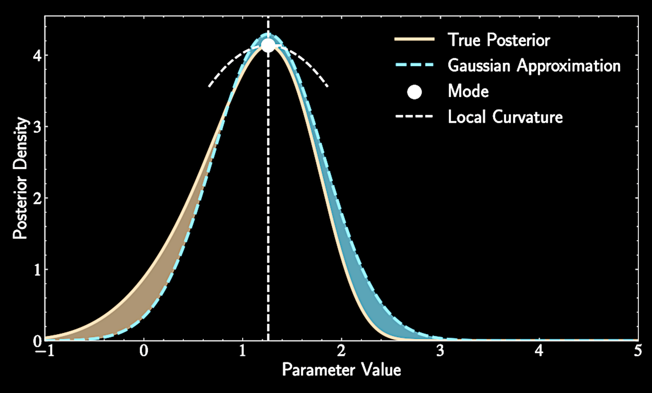
Mechanics of Laplace Approximation
We approximate our complex posterior with a Gaussian
Location of the peak (mode): becomes the mean of our approximating Gaussian
Curvature at the peak: determines covariance (measured by second derivatives of log posterior)
Dealing With Unnormalized Distribution
In Bayesian inference, we often know distributions only up to a normalization constant: \(p(z) = \frac{f(z)}{Z}\), where \(Z = \int f(z) dz\)
By Bayes' theorem:
The denominator \(p(\text{data})\) (evidence) is often intractable
Laplace approximation allows us to work directly with unnormalized density \(f(z) = p(\text{data}|z)p(z) \)
p(z|\text{data}) = \frac{p(\text{data}|z)p(z)}{p(\text{data})}
Finding the Mode of the Target Distribution
Locate the mode \(z_0\) where probability density is maximum
At this point, the derivative equals zero:
Equivalently, the derivative of log-density equals zero:
\left.\frac{d}{dz}f(z)\right|_{z=z_0} = 0
\left.\frac{d}{dz}\ln f(z)\right|_{z=z_0} = 0
Taylor Expansion Around the Mode
Second-order Taylor expansion of log-density around mode \(z_0\):
Define curvature parameter: \(A = -\left.\frac{d^2}{dz^2}\ln f(z)\right|_{z=z_0}\)
\ln f(z) \approx \ln f(z_0) + \left.\frac{d}{dz}\ln f(z)\right|_{z=z_0}(z-z_0)
+ \frac{1}{2}\left.\frac{d^2}{dz^2}\ln f(z)\right|_{z=z_0}(z-z_0)^2
Constructing the Gaussian Approximation
Approximation becomes:
Exponentiating both sides: \(f(z) \approx f(z_0)\exp\left(-\frac{1}{2}A(z-z_0)^2\right)\)
\ln f(z) \approx \ln f(z_0) - \frac{1}{2}A(z-z_0)^2
Curvature \(A\) determines the width and the normalization factor
After normalization: \(q(z) = \mathcal{N}(z|z_0, A^{-1}) \)
The Complete Laplace Approximation
Find the mode \(z_0\) of the distribution (where first derivative = zero)
Calculate second derivative at mode to determine
\(A = -\left.\frac{d^2}{dz^2}\ln f(z)\right|_{z=z_0} \)
Construct Gaussian approximation with mean \(z_0\) and variance \(A^{-1}\). We have \(q(z) = \mathcal{N}(z|z_0, A^{-1}) \)
Provides principled approach for approximating complex distributions, particularly valuable when exact posteriors are intractable
Extension to Multiple Dimensions
Step 1: Find the mode \(\mathbf{z}_0\) where the gradient of log density vanishes:
Gradient operator produces vector of partial derivatives:
\nabla \ln f(\mathbf{z})\Big|_{\mathbf{z}=\mathbf{z}_0} = \mathbf{0}
\nabla \ln f(\mathbf{z}) = \left(\frac{\partial \ln f(\mathbf{z})}{\partial z_1}, \frac{\partial \ln f(\mathbf{z})}{\partial z_2}, \ldots, \frac{\partial \ln f(\mathbf{z})}{\partial z_d}\right)^T
Multivariate Taylor Expansion
Step 2: Second-order Taylor expansion around the mode:
Hessian matrix \(\mathbf{H}\) of second derivatives:
ln f(\mathbf{z}) \approx \ln f(\mathbf{z}_0) + (\mathbf{z}-\mathbf{z}_0)^T \nabla \ln f(\mathbf{z})\Big|_{\mathbf{z}=\mathbf{z}_0}
H_{ij} = \frac{\partial^2 \ln f(\mathbf{z})}{\partial z_i \partial z_j}\Big|_{\mathbf{z}=\mathbf{z}_0}
+ \frac{1}{2}(\mathbf{z}-\mathbf{z}_0)^T \mathbf{H} (\mathbf{z}-\mathbf{z}_0)
Laplace Approximation at Multiple Dimension
Define precision matrix \(\mathbf{A} = -\mathbf{H}\) (negative Hessian)
Our approximation becomes:
\ln f(\mathbf{z}) \approx \ln f(\mathbf{z}_0) - \frac{1}{2}(\mathbf{z}-\mathbf{z}_0)^T \mathbf{A} (\mathbf{z}-\mathbf{z}_0)
Multivariate Laplace approximation is a \(\mathcal{N}(\mathbf{z}_0, \mathbf{A}^{-1})\) distribution.
Application to Bayesian Logistic Regression
MAP finds parameter values that maximize posterior probability:
Extends Maximum Likelihood Estimation by incorporating prior
\mathbf{w}_{\text{MAP}} = \arg\max_{\mathbf{w}} p(\mathbf{w}|\mathcal{D}) = \arg\max_{\mathbf{w}} {p(\mathcal{D}|\mathbf{w})p(\mathbf{w})}
When prior is uniform, MAP reduces to MLE
Then, calculate the Hessian at the log posterior evaluated at \( \mathbf{w}_{\text{MAP}} \)
The Log Posterior
Log posterior combines prior and likelihood terms:
Second term is familiar cross-entropy from MLE
\ln p(\mathbf{w}|\mathbf{t},\mathbf{X}) = \ln p(\mathbf{w}) + \ln p(\mathbf{t}|\mathbf{w},\mathbf{X})
= -\frac{1}{2}(\mathbf{w}-\mathbf{m}_0)^T\mathbf{S}_0^{-1}(\mathbf{w}-\mathbf{m}_0)
+ \sum_{n=1}^N [t_n\ln\sigma(\mathbf{w}^T\mathbf{x}_n) + (1-t_n)\ln(1-\sigma(\mathbf{w}^T\mathbf{x}_n))]
Finding the MAP Estimate
Need to optimize posterior probability using stochastic gradient descent
Computing the gradient:
\nabla \ln p(\mathbf{w}|\mathbf{t},\mathbf{X}) = \nabla \ln p(\mathbf{w}) + \nabla \ln p(\mathbf{t}|\mathbf{w},\mathbf{X})
= -\mathbf{S}_0^{-1}(\mathbf{w}-\mathbf{m}_0) + \sum_{n=1}^N (t_n - \sigma(\mathbf{w}^T\mathbf{x}_n))\mathbf{x}_n
Prior acts as regularizer that pulls weights toward \(\mathbf{m}_0\)
Finding the MAP Estimate
Unlike linear regression, no closed-form solution
Maximize log posterior \( \ln p(\mathbf{w}|\mathbf{t},\mathbf{X}) \) using SGD:
We climb up the posterior with the gradient:
\mathbf{w}^{(t+1)} = \mathbf{w}^{(t)} + \eta \nabla \ln p(\mathbf{w}^{(t)}|\mathbf{t},\mathbf{X})
After finding \(\mathbf{w}_{\text{MAP}}\), compute Hessian matrix for
Laplace approximation
Computing the Hessian Matrix
For Laplace approximation, we need negative Hessian at \(\mathbf{w}_{\text{MAP}}\)
Hessian is matrix of second derivatives of log posterior:
\mathbf{A} = \left. - \mathbf{H} \right|_{\mathbf{w}_\text{MAP}} = \left. - \nabla\nabla \ln p(\mathbf{w}) - \nabla\nabla \ln p(\mathbf{t}|\mathbf{w},\mathbf{X}) \right|_{\mathbf{w}_{\text{MAP}}}
=\mathbf{S}_0^{-1} + \sum_{n=1}^N \sigma(\mathbf{w}_{\text{MAP}}^T\mathbf{x}_n)(1-\sigma(\mathbf{w}_{\text{MAP}}^T\mathbf{x}_n))\mathbf{x}_n\mathbf{x}_n^T
Represents inverse covariance of posterior approximation
Computing the Hessian Matrix
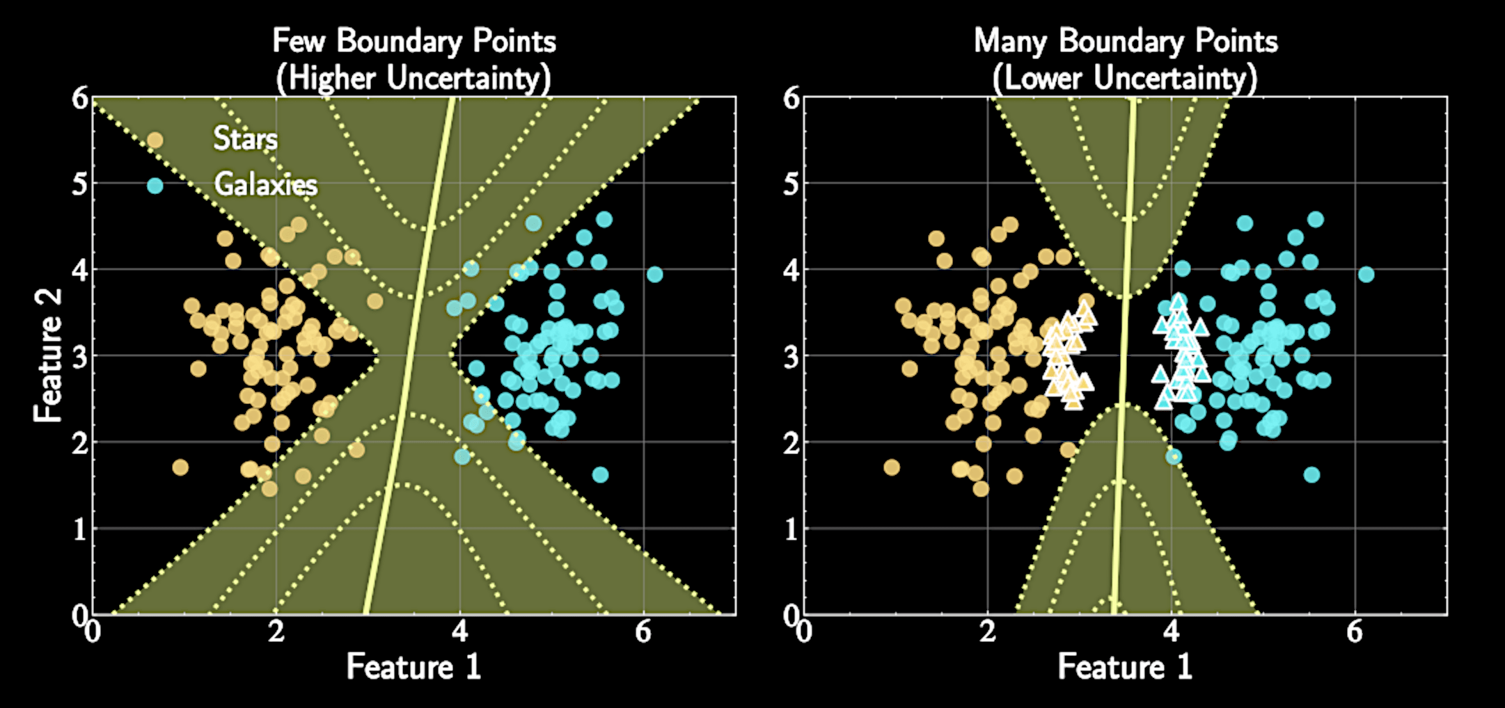
Each data point's contribution weighted by
\(\sigma(\mathbf{w}_{\text{MAP}}^T\mathbf{x}_n)(1-\sigma(\mathbf{w}_{\text{MAP}}^T\mathbf{x}_n))\)
This term has maximum value of 0.25 when \(\sigma(\mathbf{w}_{\text{MAP}}^T\mathbf{x}_n) = 0.5\) (at decision boundary)
More data points near decision boundary → increased precision matrix magnitude → less parameter uncertainty
\mathbf{A} = \mathbf{S}_0^{-1} + \sum_{n=1}^N \sigma(\mathbf{w_{\text{MAP}}}^T\mathbf{x}_n)(1-\sigma(\mathbf{w}_{\text{MAP}}^T\mathbf{x}_n))\mathbf{x}_n\mathbf{x}_n^T
Logistics
Homework Assignment 3 due this Friday,11:59pm
Select and submit your topic for group project 2 (on Carmen), by next Friday, 11:59pm
I will be away next week. Lecture will be recorded and posted on Carmen
From Posterior to Prediction
We approximated the posterior as a Gaussian distribution
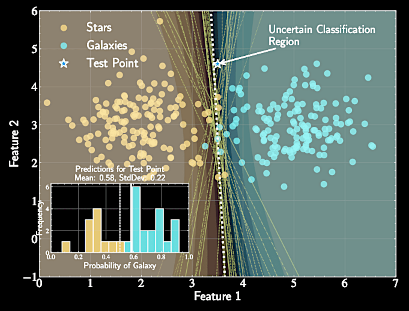
Distribution over decision boundaries: Each sample \(\mathbf{w}\) corresponds to a different boundary, assigning different probabilities
q(\mathbf{w}) = \mathcal{N}(\mathbf{w} | \mathbf{w}_{\text{MAP}}, \mathbf{A}^{-1})
\mathbf{A} = \mathbf{S}_0^{-1} + \sum_{n=1}^N \sigma(\mathbf{w_{\text{MAP}}}^T\mathbf{x}_n)(1-\sigma(\mathbf{w}_{\text{MAP}}^T\mathbf{x}_n))\mathbf{x}_n\mathbf{x}_n^T
The Predictive Distribution
Probability of a class label for a new input that integrates over all model uncertainty
A weighted average where each model contributes according to its posterior probability
p(y^* = 1 | \mathbf{x}^*, \mathcal{D}) = \int p(y^* = 1 | \mathbf{x}^*, \mathbf{w}) p(\mathbf{w} | \mathcal{D}) d\mathbf{w}
For the other class
p(y^* = 0 | \mathbf{x}^*, \mathcal{D}) = 1 - p(y^* = 1 | \mathbf{x}^*, \mathcal{D})
Computational challenge of the integral
Substituting our Gaussian approximation:
The integral lacks a closed-form solution unlike in Bayesian Linear Regression
p(y^* = 1 | \mathbf{x}^*, \mathcal{D}) \approx \int \sigma(\mathbf{w}^T \mathbf{x}^*) \mathcal{N}(\mathbf{w} | \mathbf{w}_{\text{MAP}}, \mathbf{A}^{-1}) d\mathbf{w}
Approximate sigmoid with probit function to make the integral more manageable
Simplifying the High-Dimensional Integral
For classification, what truly matters is the logit value \( a = \mathbf{w}^T \mathbf{x}^* \)
This single value determines class probability through the sigmoid function \( \sigma(a) \)
\( a \) represents signed distance from test point to decision boundary
Many different weight vectors \( \mathbf{w} \) can produce the same logit value \( a \) for a given input
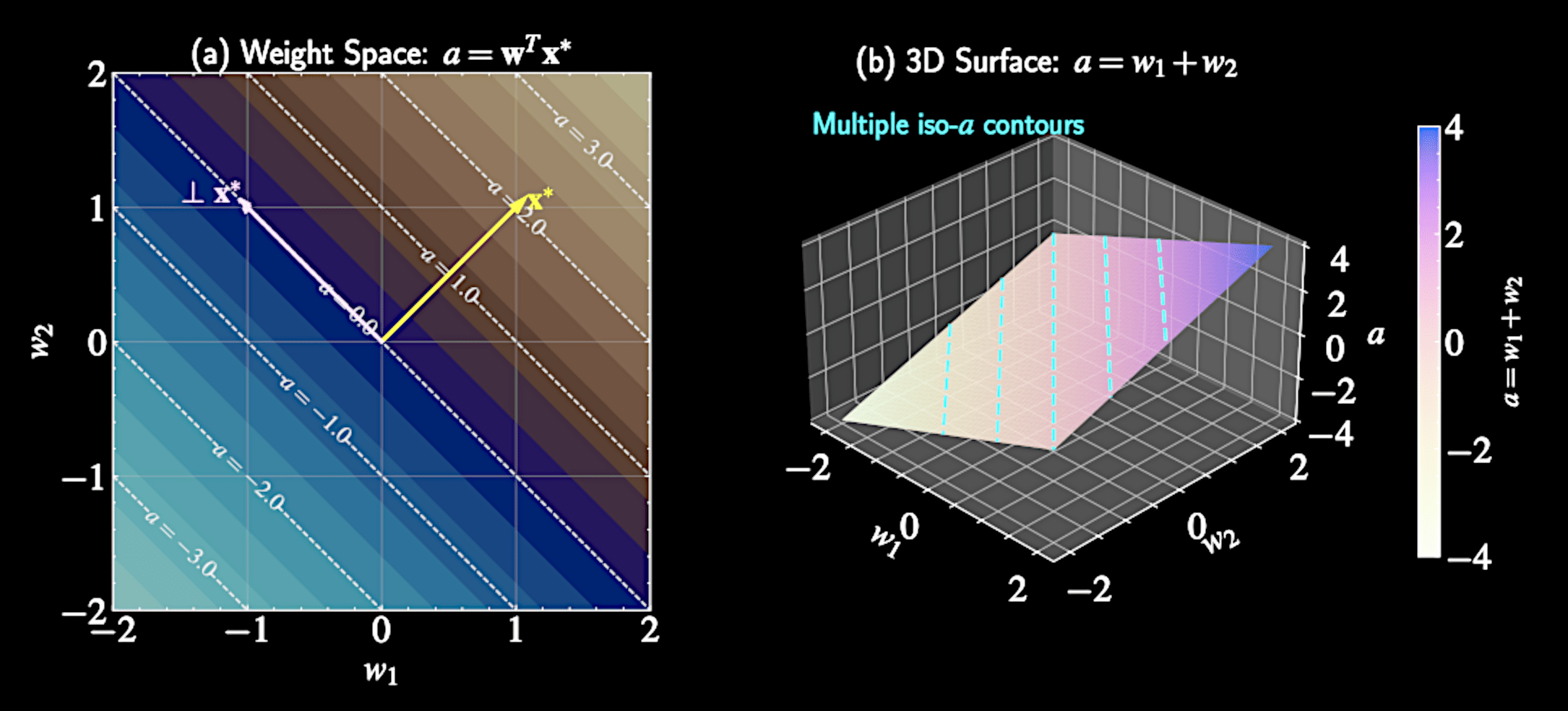
Weight Space Redundancy
Weight vectors forming a hyperplane perpendicular to \( \mathbf{x}^* \) all map to the same logit \( a \)
This many-to-one mapping suggests we can simplify by focusing on distribution of \( a \) rather than full distribution of \( \mathbf{w} \)
Decompose weight vector into components parallel and perpendicular to \( \mathbf{x}^* \): \( \mathbf{w} = w_{\parallel}\frac{\mathbf{x}^*}{|\mathbf{x}^*|} + \mathbf{w}_{\perp} \)
Only the component of \( \mathbf{w} \) parallel to \( \mathbf{x}^* \) affects the prediction. From D dimension to 1D.
Transforming the Integral
Original predictive distribution:
Change of variables from \( \mathbf{w} \) to \( ( a, \mathbf{w}_{\perp} ) \)
p(y^* = 1 | \mathbf{x}^*, \mathcal{D}) \approx \int \sigma(\mathbf{w}^T \mathbf{x}^*) \mathcal{N}(\mathbf{w} | \mathbf{w}_{\text{MAP}}, \mathbf{A}^{-1}) d\mathbf{w}
p(y^* = 1 | \mathbf{x}^*, \mathcal{D}) \approx \int \sigma(a) \mathcal{N}(a | \mu_a, \sigma_a^2) da
Transformation of Random Variables
Since \( \mathbf{w} \) follows Gaussian \( \mathcal{N}(\mathbf{w}_{\text{MAP}}, \mathbf{A}^{-1}) \), and \( a = \mathbf{w}^T \mathbf{x}^* \) is a linear combination
Linear transformations of Gaussian variables remain Gaussian
Mean and variance of logit distribution: \( \mu_a = \mathbf{w}_{\text{MAP}}^T\mathbf{x}^* \)
\( \sigma_a^2 = \mathbf{x}^{*T}\mathbf{A}^{-1}\mathbf{x}^* \)
Remarkable simplification: High-dimensional integral reduced to one-dimensional
The Probit Function
p(y^* = 1 | \mathbf{x}^*, \mathcal{D}) \approx \int \sigma(a) \mathcal{N}(a | \mu_a, \sigma_a^2) da
Mathematical forms of sigmoid and Gaussian don't allow direct integration
Need a creative approach: Replace sigmoid with a similar function
Use the probit function that allows analytical integration
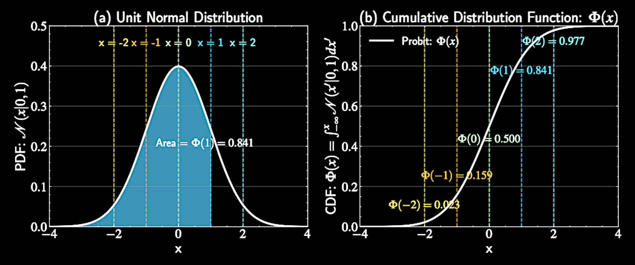
Introducing the Probit Function
Probit function \( \Phi(x) \): Cumulative distribution function (CDF) of a standard unit Gaussian distribution
Mathematical definition:
Monotonically increasing with "S" shape
\Phi(x) = \int_{-\infty}^{x} \mathcal{N}(t | 0, 1) dt
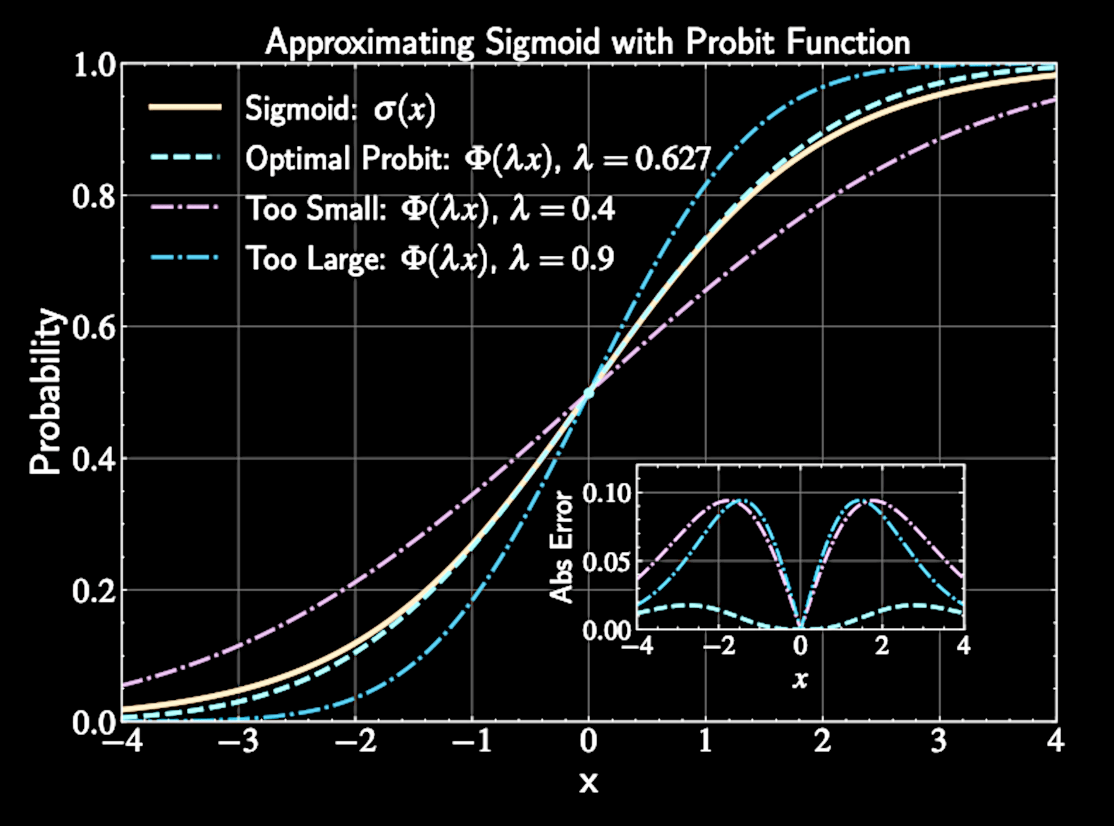
Approximating Sigmoid with Probit
Need to approximate: \( \sigma(a) \approx \Phi(\lambda a) \)
Find optimal \( \lambda \) by equating derivatives at \( a = 0 \):
Sigmoid derivative at origin: \( \frac{d}{da}\sigma(a)|_{a=0} = \frac{1}{4} \). Probit derivative at origin: \( \frac{d}{da}\Phi(\lambda a)|_{a=0} = \frac{\lambda}{\sqrt{2\pi}} \)
Equating these: \( \frac{1}{4} = \frac{\lambda}{\sqrt{2\pi}} \implies \lambda = \sqrt{\frac{\pi}{8}} \approx 0.63 \)
The Key Mathematical Property
Remarkable property of probit function when integrated with Gaussian:
This identity is exactly what we need to solve our predictive distribution integral
Can be proven elegantly using properties of random variables
\int \Phi(\lambda a) \mathcal{N}(a | \mu, \sigma^2) da = \Phi\left(\frac{\lambda\mu}{\sqrt{1 + \lambda^2\sigma^2}}\right)
Proving the Identity
Consider two independent random variables:
Linear combination of random variables \( \)
\( X \sim \mathcal{N}(0, 1/\lambda^2) \)
\( Y \sim \mathcal{N}(\mu, \sigma^2) \)
X - Y \sim \mathcal{N}(-\mu, 1/\lambda^2 + \sigma^2)
Proving the Identity
Probability that \( P(X < Y) \) or \( P( X - Y < 0 ) \) is:
Definition of the Probit function and cumulative distribution function
P(X - Y < 0) = \Phi\left(\frac{\mu}{\sqrt{1/\lambda^2 + \sigma^2}}\right) = \Phi\left(\frac{\lambda\mu}{\sqrt{1 + \lambda^2\sigma^2}}\right)
X - Y \sim \mathcal{N}(-\mu, 1/\lambda^2 + \sigma^2)
\int \Phi(\lambda a) \mathcal{N}(a | \mu, \sigma^2) da = \Phi\left(\frac{\lambda\mu}{\sqrt{1 + \lambda^2\sigma^2}}\right)
The RHS of
Proving the Identity
Calculate same probability by conditioning on value of \( Y \)
For each possible \( y \), probability that \( X < y \) is \( \Phi(\lambda y) \)
Integrate over all possible values
This gives us: \( P(X < Y) = \int_{-\infty}^{\infty} \Phi(\lambda y) \mathcal{N}(y | \mu, \sigma^2) dy \). Equals to the LHS of the identity
\int \Phi(\lambda a) \mathcal{N}(a | \mu, \sigma^2) da = \Phi\left(\frac{\lambda\mu}{\sqrt{1 + \lambda^2\sigma^2}}\right)
Derivation of the Predictive Distribution
Original predictive distribution integral:
Using probit approximation:
p(y^* = 1 | \mathbf{x}^*, \mathcal{D}) = \int \sigma(\mathbf{w}^T\mathbf{x}^*) p(\mathbf{w}|\mathcal{D}) d\mathbf{w}
p(y^* = 1 | \mathbf{x}^*, \mathcal{D}) = \int \sigma(a) \mathcal{N}(a | \mu_a, \sigma_a^2) da
p(y^* = 1 | \mathbf{x}^*, \mathcal{D}) \approx \int \Phi\left(\sqrt{\frac{\pi}{8}} a\right) \mathcal{N}(a | \mu_a, \sigma_a^2) da
Applying the Integration Formula
Using our derived identity with \( \lambda = \sqrt{\pi/8} \):
Converting back to sigmoid function:
\int \Phi\left(\sqrt{\frac{\pi}{8}} a\right) \mathcal{N}(a | \mu_a, \sigma_a^2) da = \Phi\left(\frac{\sqrt{\pi/8} \cdot \mu_a}{\sqrt{1 + (\pi/8) \sigma_a^2}}\right)
\Phi\left(\frac{\sqrt{\pi/8} \cdot \mu_a}{\sqrt{1 + (\pi/8) \sigma_a^2}}\right) \approx \sigma\left(\frac{\mu_a}{\sqrt{1 + \pi\sigma_a^2/8}}\right)
Final expression for predictive distribution:
Where \( \mu_a = \mathbf{w}_{\text{MAP}}^T\mathbf{x}^* \) and \( \sigma_a^2 = \mathbf{x}^{*T}\mathbf{A}^{-1}\mathbf{x}^* \)
p(y^* = 1 | \mathbf{x}^*, \mathcal{D}) \approx \sigma\left(\frac{\mu_a}{\sqrt{1 + \pi\sigma_a^2/8}}\right)
p(y^* = 1 | \mathbf{x}^*, \mathcal{D}) \approx \sigma\left(\kappa(\mathbf{x}^{*T} \mathbf{A}^{-1} \mathbf{x}^*) \cdot \mathbf{w}_{\text{MAP}}^T \mathbf{x}^*\right)
Substituting original terms:
Define uncertainty factor: \( \kappa(\sigma_a^2) = (1 + \pi\sigma_a^2/8)^{-1/2} \)
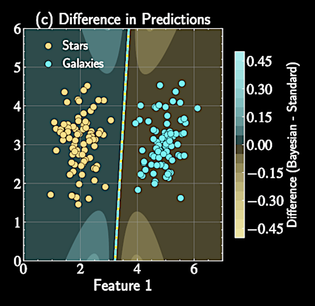
Comparison with Standard Logistic Regression
Dampens certainty of predictions by pushing toward 0.5
p(y^* = 1 | \mathbf{x}^*, \mathcal{D}) \approx \sigma\left(\kappa(\mathbf{x}^{*T} \mathbf{A}^{-1} \mathbf{x}^*) \cdot \mathbf{w}_{\text{MAP}}^T \mathbf{x}^*\right)
Standard logistic regression prediction:
Uncertainty factor: \( \kappa(\sigma_a^2) = (1 + \pi\sigma_a^2/8)^{-1/2} \)
p(y^* = 1 | \mathbf{x}^*, \mathbf{w}_{\text{MAP}}) = \sigma(\mathbf{w}_{\text{MAP}}^T \mathbf{x}^*)
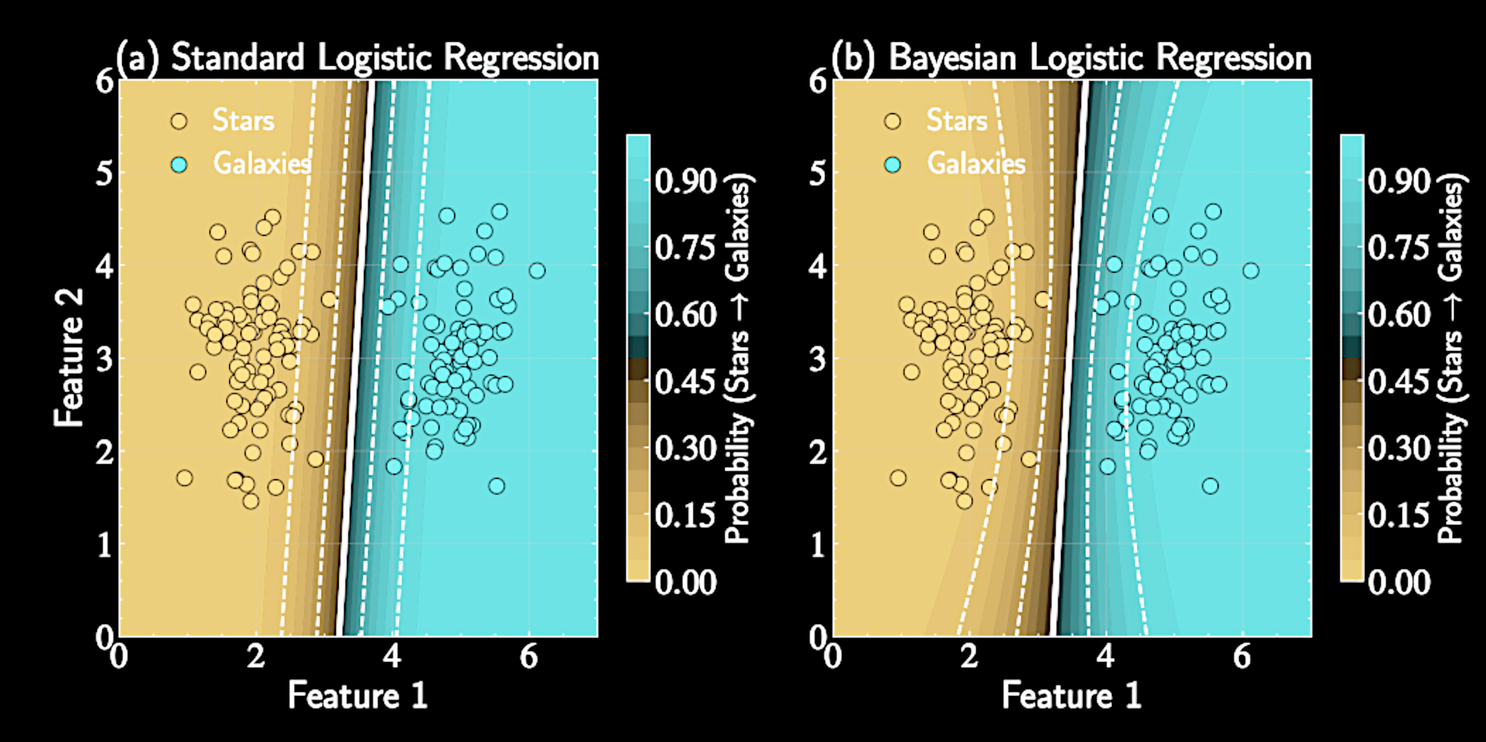
Geometric Interpretation of Uncertainty
When \( \mathbf{x}^* \) is far from training data \(\rightarrow\) Larger values in \( \mathbf{A}^{-1} \) in direction of \( \mathbf{x}^* \)
The variance \( \sigma_a^2 = \mathbf{x}^{*T} \mathbf{A}^{-1} \mathbf{x}^* \) depends on the location of test point relative to training data
Uncertainty factor: \( \kappa(\sigma_a^2) = (1 + \pi\sigma_a^2/8)^{-1/2} \)
Increased \( \sigma_a^2 \) reflecting greater uncertainty. Boundary becomes "softer" away from training data
Application to Astronomical Classification
Bayesian approach provides crucial uncertainty signal.
Naturally conservative with unusual objects
Predictions closer to 0.5 for objects unlike training examples
Identifies potential new or transitional types
What We Have Learned
Bayesian Logistic Regression
Soft Boundary
Laplace Approximation
Probit Approximation
Astron 5550 - Lecture 9
By Yuan-Sen Ting


