CS 106A
Stanford University
Chris Gregg
Using Python for Artificial Intelligence
Today's topics:
Introduction to Artificial Intelligence
Introduction to Artificial Neural Networks
Examples of some basic neural networks
Using Python for Artificial Intelligence
Example: PyTorch
Using Python for Artificial Intelligence
1950: Alan Turing: Turing Test
1951: First AI program
1965: Eliza (first chat bot)
1974: First autonomous vehicle
1997: Deep Blue beats Gary Kasimov at Chess
2004: First Autonomous Vehicle challenge
2011: IBM Watson beats Jeopardy winners
2016: Deep Mind beats Go champion
2017: AlphaGo Zero beats Deep Mind
Introduction to Artificial Intelligence
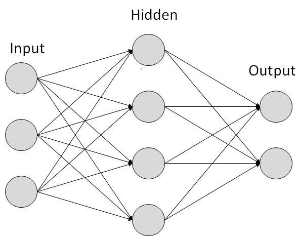
NNs learn relationship between cause and effect or organize large volumes of data into orderly and informative patterns.
Introduction to Artificial Neural Networks (ANNs)
Slides modified from PPT by Mohammed Shbier
- A Neural Network is a biologically inspired information processing idea, modeled after our brain.
- A neural network is a large number of highly interconnected processing elements (neurons) working together
- Like people, they learn from experience (by example)
Introduction to Artificial Neural Networks (ANNs)
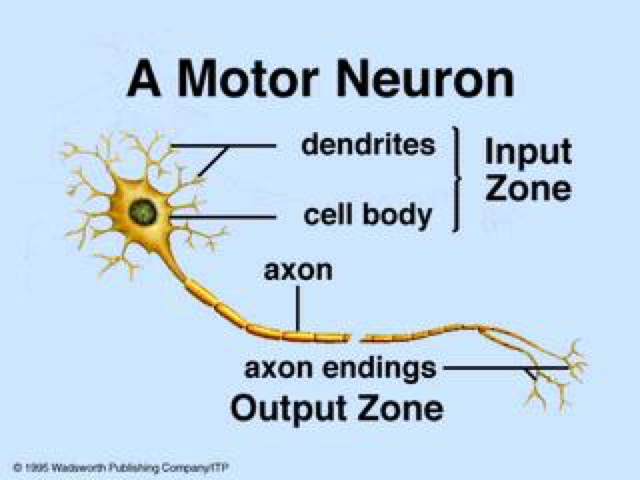
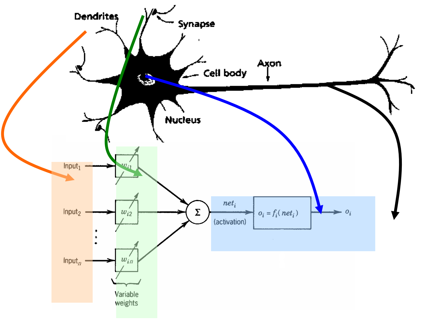
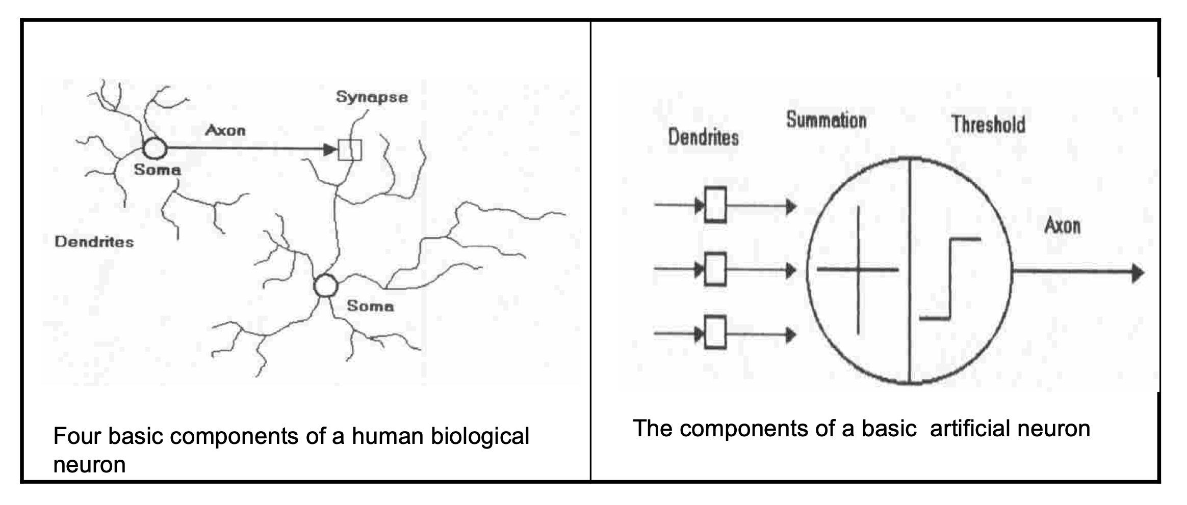
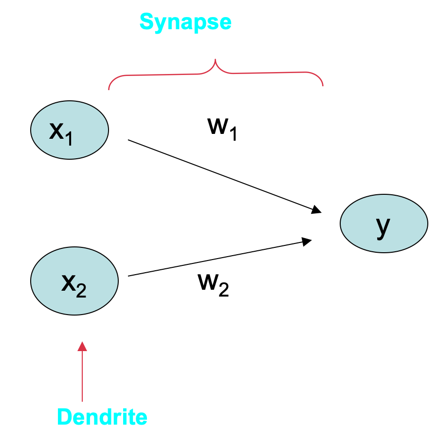
- Neural networks take their inspiration from neurobiology
- This diagram is the human neuron:
Introduction to Artificial Neural Networks (ANNs)
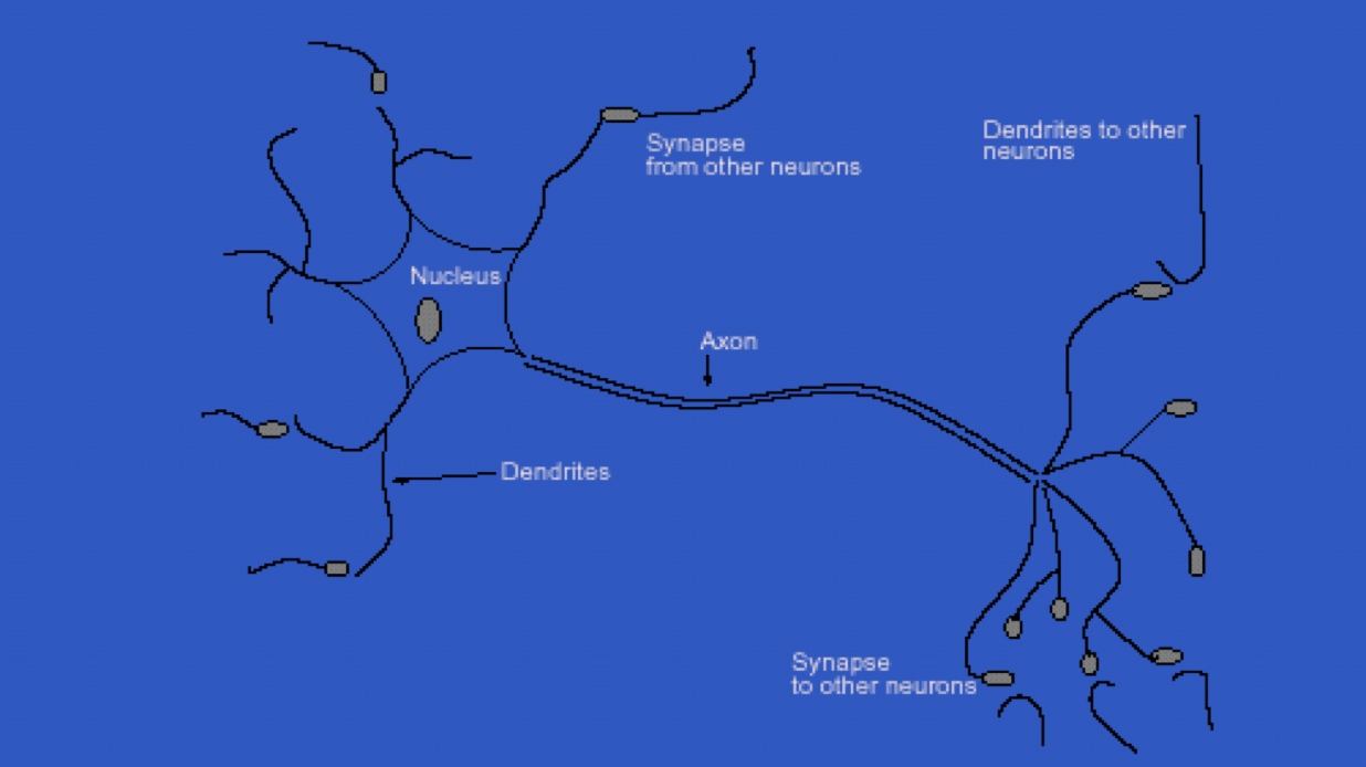
- A biological neuron has three types of main components; dendrites, soma (or cell body) and axon
- Dendrites receives signals from other neurons
- The soma, sums the incoming signals. When sufficient input is received, the cell fires; that is it transmit a signal over its axon to other cells.
Introduction to Artificial Neural Networks (ANNs)
- An artificial neural network (ANN) is an information processing system that has certain performance characteristics in common with biological nets.
- Several key features of the processing elements of ANN are suggested by the properties of biological neurons:
Introduction to Artificial Neural Networks (ANNs)
-
The processing element receives many signals.
-
Signals may be modified by a weight at the receiving synapse.
-
The processing element sums the weighted inputs.
-
Under appropriate circumstances (sufficient input), the neuron transmits a single output.
-
The output from a particular neuron may go to many other neurons.
- From experience: examples / training data
- Strength of connection between the neurons is stored as a weight-value for the specific connection.
- Learning the solution to a problem = changing the connection weights
Introduction to Artificial Neural Networks (ANNs)
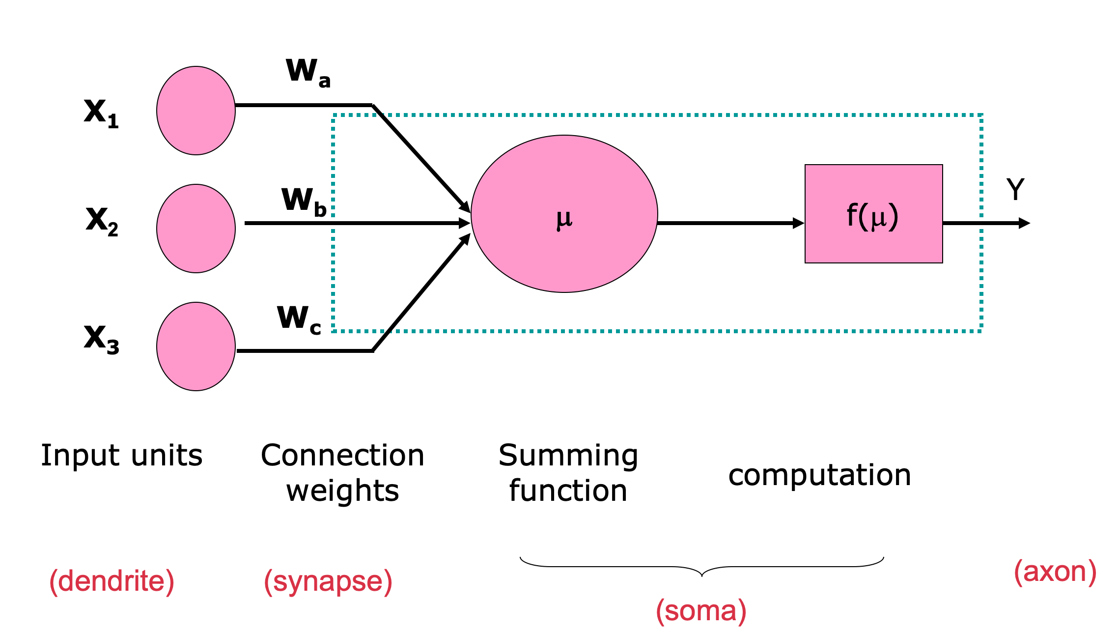
- ANNs have been developed as generalizations of mathematical models of neural biology, based on the assumptions that:
- Information processing occurs at many simple elements called neurons.
- Signals are passed between neurons over connection links.
- Each connection link has an associated weight, which, in typical neural net, multiplies the signal transmitted.
- Each neuron applies an activation function to its net input to determine its output signal.
Introduction to Artificial Neural Networks (ANNs)
Introduction to Artificial Neural Networks (ANNs)
- Model of a neuron
Introduction to Artificial Neural Networks (ANNs)
-
A neural net consists of a large number of simple processing elements called neurons, units, cells or nodes.
-
Each neuron is connected to other neurons by means of directed communication links, each with associated weight.
-
The weight represent information being used by the net to solve a problem.
-
Each neuron has an internal state, called its activation or activity level, which is a function of the inputs it has received. Typically, a neuron sends its activation as a signal to several other neurons.
-
It is important to note that a neuron can send only one signal at a time, although that signal is broadcast to several other neurons.
Introduction to Artificial Neural Networks (ANNs)
-
Neural networks are configured for a specific application, such as pattern recognition or data classification, through a learning process
-
In a biological system, learning involves adjustments to the synaptic connections between neurons
-
This is the same for artificial neural networks (ANNs)!
Introduction to Artificial Neural Networks (ANNs)
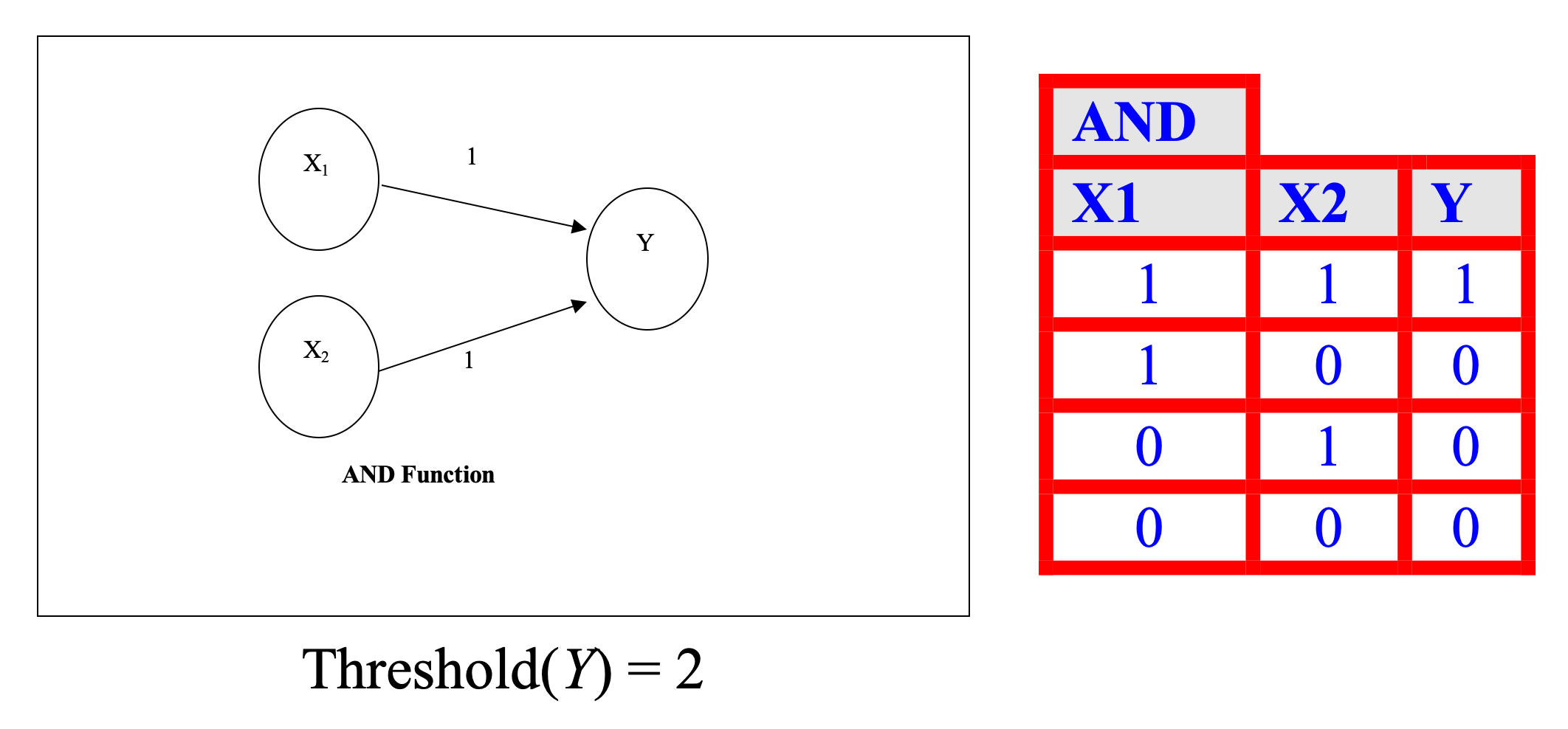
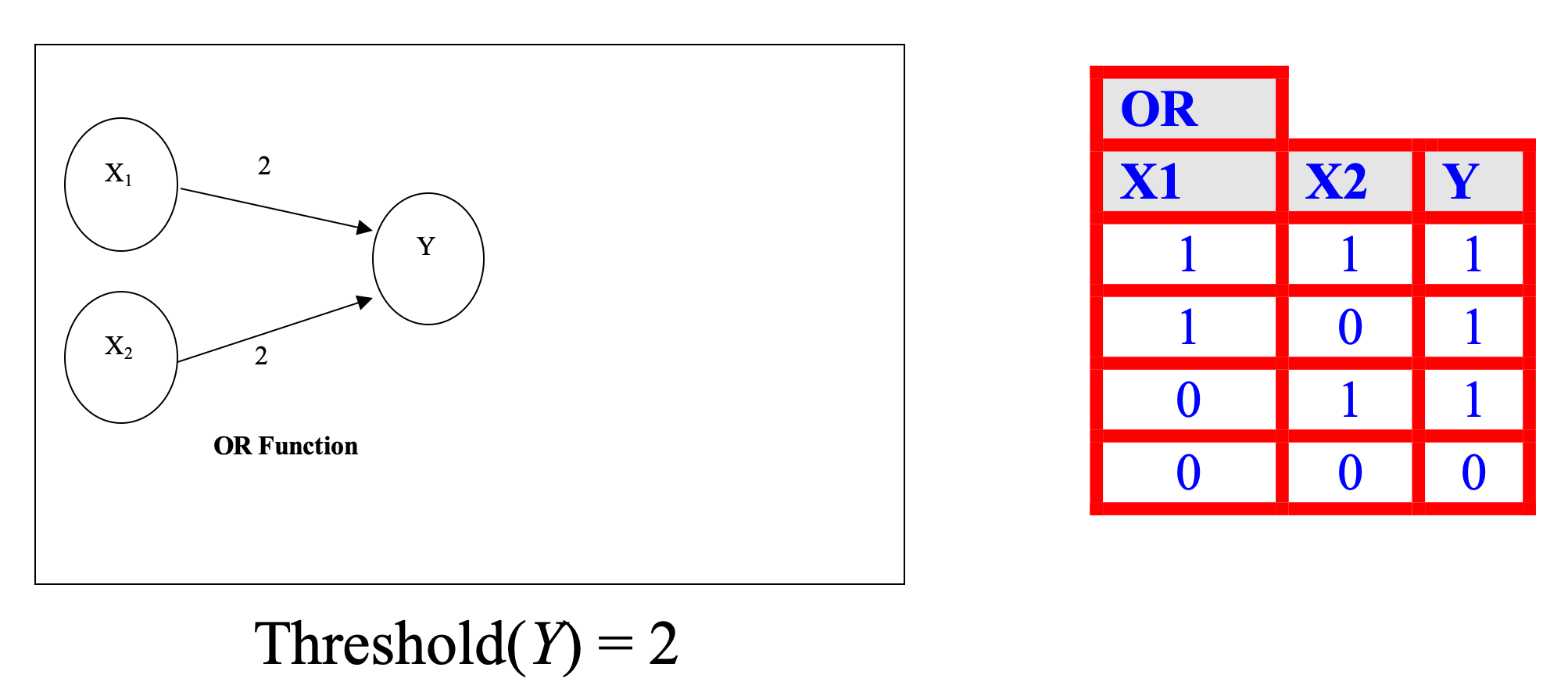
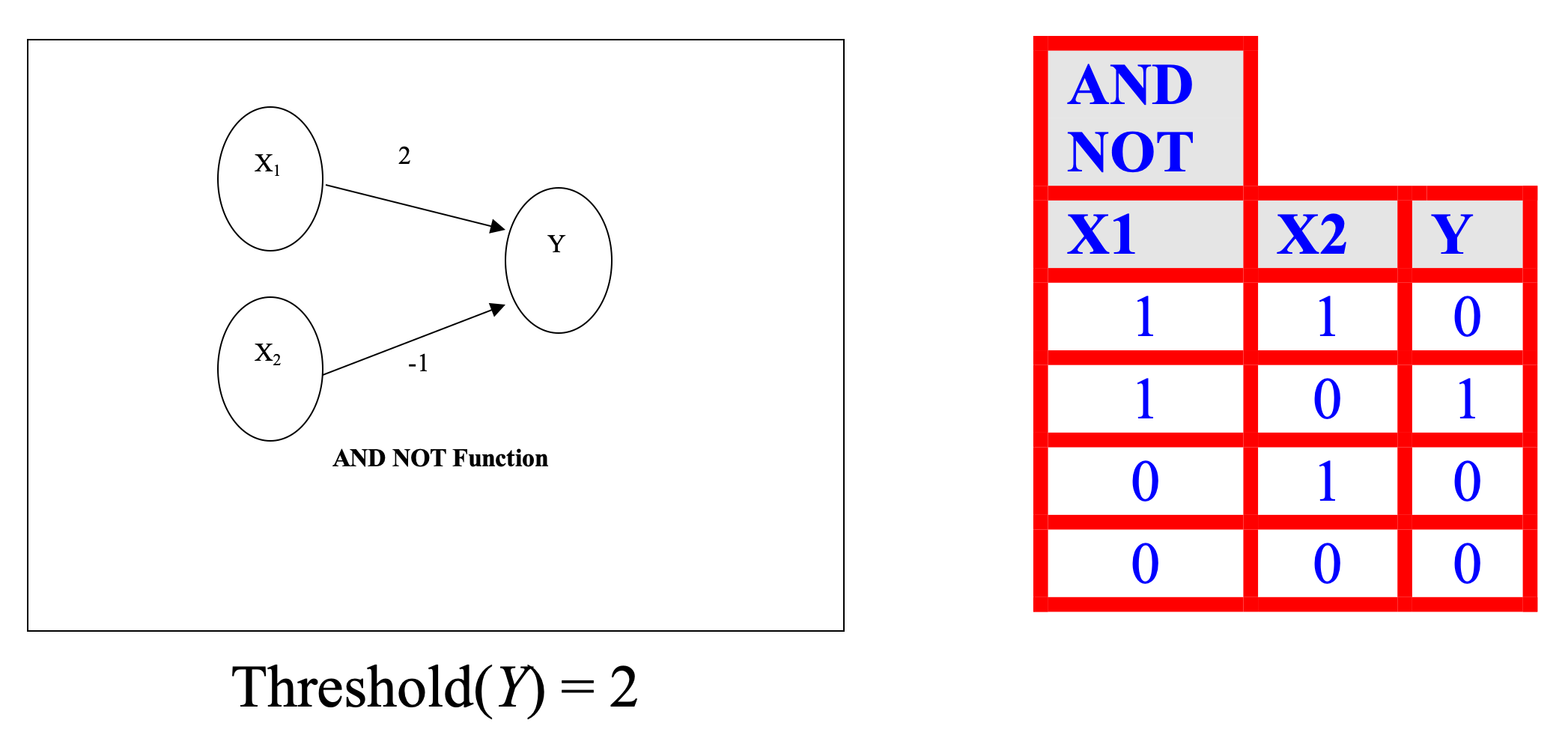
- A neuron receives input, determines the strength or the weight of the input, calculates the total weighted input, and compares the total weighted with a value (threshold)
- The value is in the range of 0 and 1
- If the total weighted input greater than or equal the threshold value, the neuron will produce the output, and if the total weighted input less than the threshold value, no output will be produced
Introduction to Artificial Neural Networks (ANNs)
Introduction to Artificial Neural Networks (ANNs)
Introduction to Artificial Neural Networks (ANNs)
Introduction to Artificial Neural Networks (ANNs)
Introduction to Artificial Neural Networks (ANNs)
Introduction to Artificial Neural Networks (ANNs)
Let's model a slightly more complicated neural network:
-
If we touch something cold we perceive heat
-
If we keep touching something cold we will perceive cold
-
If we touch something hot we will perceive heat
- We will assume that we can only change things on discrete time steps
-
If cold is applied for one time step then heat will be perceived
-
If a cold stimulus is applied for two time steps then cold will be perceived
-
If heat is applied at a time step, then we should perceive heat
Introduction to Artificial Neural Networks (ANNs)
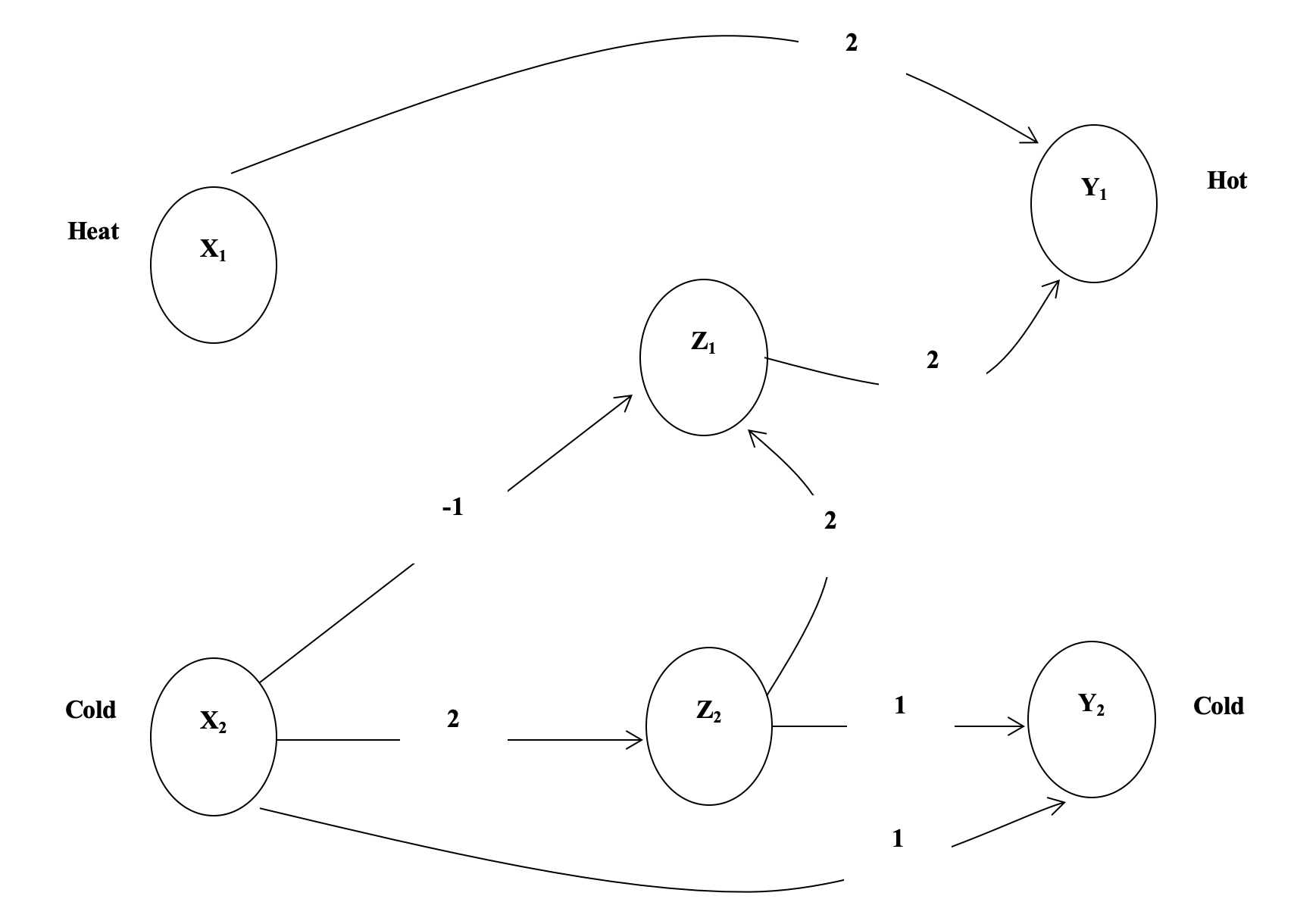
Introduction to Artificial Neural Networks (ANNs)
- It takes time for the stimulus (applied at X1 and X2) to make its way to Y1 and Y2 where we perceive either heat or cold
-
At t(0), we apply a stimulus to X1 and X2
-
At t(1) we can update Z1, Z2 and Y1
-
At t(2) we can perceive a stimulus at Y2
-
At t(2+n) the network is fully functional
Introduction to Artificial Neural Networks (ANNs)
- We want the system to perceive cold if a cold stimulus is applied for two time steps
Y2(t) = X2(t – 2) AND X2(t – 1)
| X2(t – 2) | X2( t – 1) | Y2(t) |
|---|---|---|
| 1 | 1 | 1 |
| 1 | 0 | 0 |
| 0 | 1 | 0 |
| 0 | 0 | 0 |
Introduction to Artificial Neural Networks (ANNs)
- We want the system to perceive heat if either a hot stimulus is applied or a cold stimulus is applied (for one time step) and then removed
Y1(t) = [ X1(t – 1) ] OR [ X2(t – 3) AND NOT X2(t – 2) ]
| X2(t – 3) | X2(t – 2) | AND NOT | X1(t – 1) | OR |
|---|---|---|---|---|
| 1 | 1 | 0 | 1 | 1 |
| 1 | 0 | 1 | 1 | 1 |
| 0 | 1 | 0 | 1 | 1 |
| 0 | 0 | 0 | 1 | 1 |
| 1 | 1 | 0 | 0 | 0 |
| 1 | 0 | 1 | 0 | 1 |
| 0 | 1 | 0 | 0 | 0 |
| 0 | 0 | 0 | 0 | 0 |
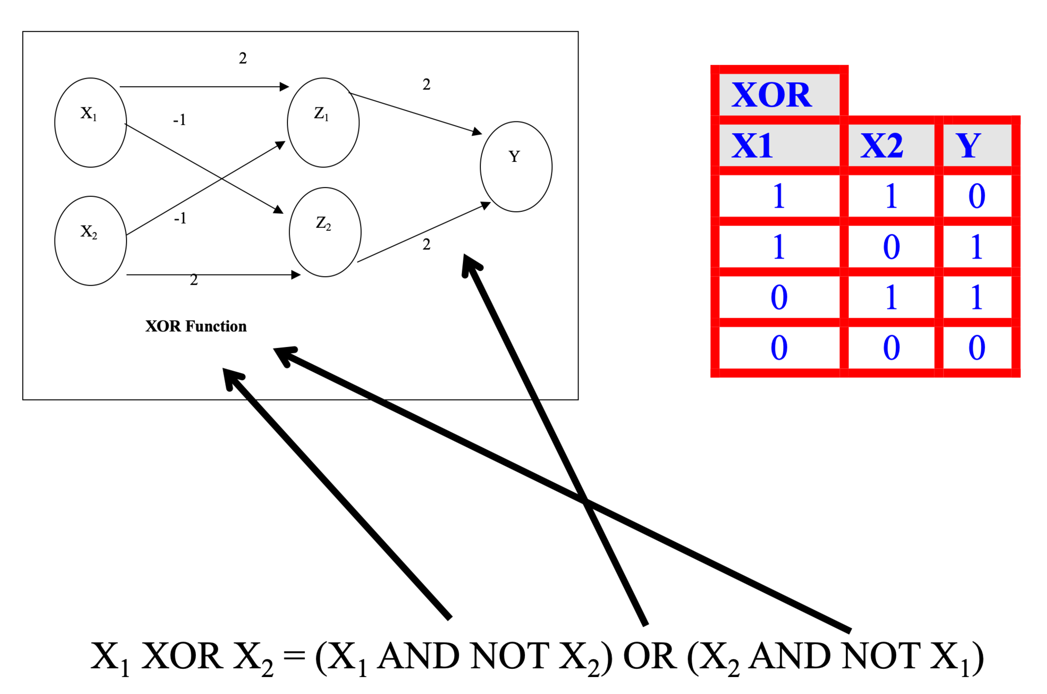
Introduction to Artificial Neural Networks (ANNs)
-
The network shows
Y1(t) = X1(t – 1) OR Z1(t – 1)
Z1(t – 1) = Z2( t – 2) AND NOT X2(t – 2)
Z2(t – 2) = X2(t – 3)
Substituting, we get
Y1(t) = [ X1(t – 1) ] OR [ X2(t – 3) AND NOT X2(t – 2) ]
which is the same as our original requirements
Using Python for Artificial Intelligence
-
This is great...but how do you build a network that learns?
-
We have to use input to predict output
-
We can do this using a mathematical algorithm called backpropagation, which measures statistics from input values and output values.
-
Backpropagation uses a training set
-
We are going to use the following training set:
Example borrowed from: How to build a simple neural network in 9 lines of Python code
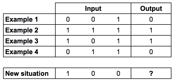
-
Can you figure out what the question mark should be?
-
This is great...but how do you build a network that learns?
-
We have to use input to predict output
-
We can do this using a mathematical algorithm called backpropogation, which measures statistics from input values and output values.
-
Backpropogation uses a training set
-
We are going to use the following training set:
Example borrowed from: How to build a simple neural network in 9 lines of Python code
-
Can you figure out what the question mark should be?
-
The output is always equal to the value of the leftmost input column. Therefore the answer is the ‘?’ should be 1.
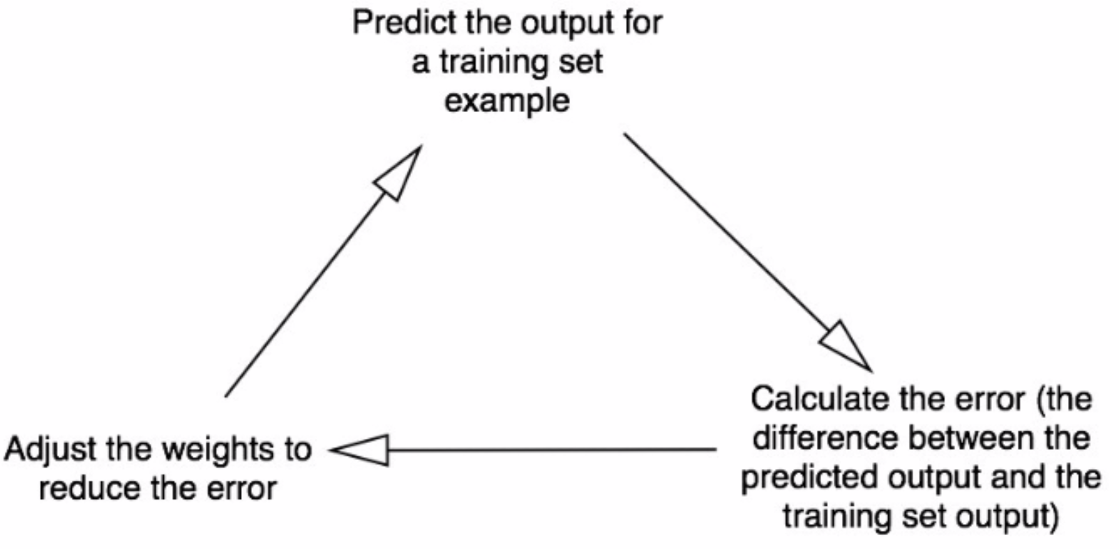
Using Python for Artificial Intelligence
-
We start by giving each input a weight, which will be a positive or negative number.
-
Large numbers (positive or negative) will have a large effect on the neuron's output.
-
We start by setting each weight to a random number, and then we train:
-
Take the inputs from a training set example, adjust them by the weights, and pass them through a special formula to calculate the neuron’s output.
-
Calculate the error, which is the difference between the neuron’s output and the desired output in the training set example.
-
Depending on the direction of the error, adjust the weights slightly.
-
Repeat this process 10,000 times.
Example borrowed from: How to build a simple neural network in 9 lines of Python code
Using Python for Artificial Intelligence
Example borrowed from: How to build a simple neural network in 9 lines of Python code
Eventually the weights of the neuron will reach an optimum for the training set. If we allow the neuron to think about a new situation, that follows the same pattern, it should make a good prediction.
Using Python for Artificial Intelligence
Example borrowed from: How to build a simple neural network in 9 lines of Python code
- What is this special formula that we're going to use to calculate the neuron's output?
- First, we take the weighted sum of the neuron's inputs:
Using Python for Artificial Intelligence
\sum{weight_i\times input_i}=weight_1\times input_1 + weight_2 \times input_2 + weight_3 \times input_3
- Next we normalize this, so the result is between 0 and 1. For this, we use a mathematically convenient function, called the Sigmoid function:
\frac{1}{1+e^{-x}}
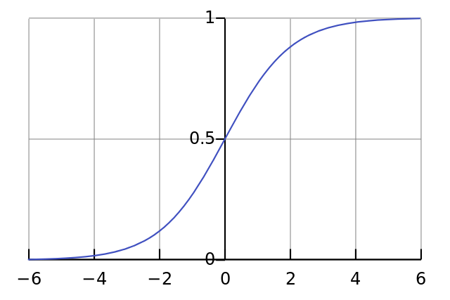
- The Sigmoid function looks like this when plotted:
- Notice the characteristic "S" shape, and that it is bounded by 1 and 0.
Example borrowed from: How to build a simple neural network in 9 lines of Python code
- We can substitute the first function into the Sigmoid:
Using Python for Artificial Intelligence
- During the training, we have to adjust the weights. To calculate this, we use the Error Weighted Derivative formula:
\frac{1}{1+e^{-\left(\sum{weight_i\times input_i}\right)}}
error \times input \times SigmoidCurvedGradient(output)
- What's going on with this formula?
- We want to make an adjustment proportional to the size of the error
- We multiply by the input, which is either 1 or 0
- We multiply by the gradient (steepness) of the Sigmoid curve.
Example borrowed from: How to build a simple neural network in 9 lines of Python code
Using Python for Artificial Intelligence
- What's going on with this formula?
- We want to make an adjustment proportional to the size of the error
- We multiply by the input, which is either 1 or 0
- We multiply by the gradient (steepness) of the Sigmoid curve.
- Why the gradient of the Sigmoid?
- We used the Sigmoid curve to calculate the output of the neuron.
- If the output is a large positive or negative number, it signifies the neuron was quite confident one way or another.
- From the diagram, we can see that at large numbers, the Sigmoid curve has a shallow gradient.
- If the neuron is confident that the existing weight is correct, it doesn’t want to adjust it very much. Multiplying by the Sigmoid curve gradient achieves this.
Example borrowed from: How to build a simple neural network in 9 lines of Python code
Using Python for Artificial Intelligence
-
The gradient of the Sigmoid curve, can be found by taking the derivative (remember calculus?)
-
So by substituting the second equation into the first equation (from two slides ago), the final formula for adjusting the weights is:
SigmoidCurvedGradient(output)=output \times (1-output)
error \times input \times output \times (1-output)
-
There are other, more advanced formulas, but this one is pretty simple.
Example borrowed from: How to build a simple neural network in 9 lines of Python code
Using Python for Artificial Intelligence
-
Finally, Python!
-
We will use the numpy module, which is a mathematics library for Python.
-
We want to use four methods:
- exp — the natural exponential
- array — creates a matrix
- dot — multiplies matrices
- random — gives us random numbers
array() creates list-like arrays that are faster than regular lists. E.g., for the training set we saw earlier:
training_set_inputs = array([[0, 0, 1], [1, 1, 1], [1, 0, 1], [0, 1, 1]])
training_set_outputs = array([[0, 1, 1, 0]]).T-
The ‘.T’ function, transposes the matrix from horizontal to vertical. So the computer is storing the numbers like this:
\begin{bmatrix}
0 & 0 & 1 \\
1 & 1 & 1 \\
1 & 0 & 1 \\
0 & 1 & 1
\end{bmatrix}
\begin{bmatrix}
0 \\
1 \\
1 \\
0
\end{bmatrix}
Example borrowed from: How to build a simple neural network in 9 lines of Python code
Using Python for Artificial Intelligence
In 10 lines of Python code:
from numpy import exp, array, random, dot
training_set_inputs = array([[0, 0, 1], [1, 1, 1], [1, 0, 1], [0, 1, 1]])
training_set_outputs = array([[0, 1, 1, 0]]).T
random.seed(1)
synaptic_weights = 2 * random.random((3, 1)) - 1
for iteration in range(10000):
    output = 1 / (1 + exp(-(dot(training_set_inputs, synaptic_weights))))
    synaptic_weights += dot(training_set_inputs.T, (training_set_outputs - output)
                                                            * output * (1 - output))
print 1 / (1 + exp(-(dot(array([1, 0, 0]), synaptic_weights))))
Example borrowed from: How to build a simple neural network in 9 lines of Python code
Using Python for Artificial Intelligence
With comments, and in a Class:
from numpy import exp, array, random, dot


class NeuralNetwork():
    def __init__(self):
        # Seed the random number generator, so it generates the same numbers
        # every time the program runs.
        random.seed(1)

        # We model a single neuron, with 3 input connections and 1 output connection.
        # We assign random weights to a 3 x 1 matrix, with values in the range -1 to 1
        # and mean 0.
        self.synaptic_weights = 2 * random.random((3, 1)) - 1

    # The Sigmoid function, which describes an S shaped curve.
    # We pass the weighted sum of the inputs through this function to
    # normalise them between 0 and 1.
    def __sigmoid(self, x):
        return 1 / (1 + exp(-x))

    # The derivative of the Sigmoid function.
    # This is the gradient of the Sigmoid curve.
    # It indicates how confident we are about the existing weight.
    def __sigmoid_derivative(self, x):
        return x * (1 - x)

    # We train the neural network through a process of trial and error.
    # Adjusting the synaptic weights each time.
    def train(self, training_set_inputs, training_set_outputs, number_of_training_iterations):
        for iteration in range(number_of_training_iterations):
            # Pass the training set through our neural network (a single neuron).
            output = self.think(training_set_inputs)

            # Calculate the error (The difference between the desired output
            # and the predicted output).
            error = training_set_outputs - output

            # Multiply the error by the input and again by the gradient of the Sigmoid curve.
            # This means less confident weights are adjusted more.
            # This means inputs, which are zero, do not cause changes to the weights.
            adjustment = dot(training_set_inputs.T, error * self.__sigmoid_derivative(output))

            # Adjust the weights.
            self.synaptic_weights += adjustment

    # The neural network thinks.
    def think(self, inputs):
        # Pass inputs through our neural network (our single neuron).
        return self.__sigmoid(dot(inputs, self.synaptic_weights))


if __name__ == "__main__":

    #Intialise a single neuron neural network.
    neural_network = NeuralNetwork()

    print("Random starting synaptic weights: ")
    print(neural_network.synaptic_weights)

    # The training set. We have 4 examples, each consisting of 3 input values
    # and 1 output value.
    training_set_inputs = array([[0, 0, 1], [1, 1, 1], [1, 0, 1], [0, 1, 1]])
    training_set_outputs = array([[0, 1, 1, 0]]).T

    # Train the neural network using a training set.
    # Do it 10,000 times and make small adjustments each time.
    neural_network.train(training_set_inputs, training_set_outputs, 10000)

    print("New synaptic weights after training: ")
    print(neural_network.synaptic_weights)

    # Test the neural network with a new situation.
    print("Considering new situation [1, 0, 0] -> ?: ")
    print(neural_network.think(array([1, 0, 0])))
Too small! Let's do this in PyCharm
Example borrowed from: How to build a simple neural network in 9 lines of Python code
Using Python for Artificial Intelligence
When we run the code, we get something like this:
Random starting synaptic weights:
[[-0.16595599]
[ 0.44064899]
[-0.99977125]]

New synaptic weights after training:
[[ 9.67299303]
[-0.2078435 ]
[-4.62963669]]

Considering new situation [1, 0, 0] -> ?:
[ 0.99993704]- First the neural network assigned itself random weights, then trained itself using the training set. Then it considered a new situation [1, 0, 0] and predicted 0.99993704. The correct answer was 1. So very close!
- This was one neuron doing one task, but if we had millions of these working together, we could create a much more robust network!
Example: PyTorch
- The example we just finished is pretty tiny, and involves only one neuron.
- If we want to do more powerful neural networks, we should use a library. One of the most widely used machine learning library is called PyTorch, and it is open source and available for many platforms.
- PyTorch allows you to use Graphics Processing Units (GPUs) for doing the substantial processing necessary for large machine learning problems
- We will take a look at part of a PyTorch tutorial, located at
https://pytorch.org/tutorials/beginner/deep_learning_60min_blitz.html
Example: PyTorch
- We are going to use PyTorch to build a straightforward image classifier, that will attempt to tell what kind of thing is in an image.
- The images are from the "CIFAR10" dataset. It has the classes you can see to the
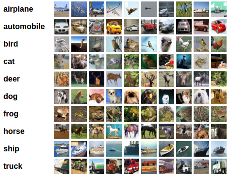
right. The images in CIFAR-10 are of size 3x32x32, i.e. 3-channel color images of 32x32 pixels in size (pretty small and blurry!)
Example: PyTorch
To train the classifier, we will do the following steps in order:
- Load and normalizing the CIFAR10 training and test datasets using torchvision
- Define a Convolutional Neural Network
- Define a loss function
- Train the network on the training data
- Test the network on the test data
Example: PyTorch
First, we'll load the data:
import torch
import torchvision
import torchvision.transforms as transforms

transform = transforms.Compose(
    [transforms.ToTensor(),
     transforms.Normalize((0.5, 0.5, 0.5), (0.5, 0.5, 0.5))])

trainset = torchvision.datasets.CIFAR10(root='./data', train=True,
                                        download=True, transform=transform)
trainloader = torch.utils.data.DataLoader(trainset, batch_size=4,
                                          shuffle=True, num_workers=2)

testset = torchvision.datasets.CIFAR10(root='./data', train=False,
                                       download=True, transform=transform)
testloader = torch.utils.data.DataLoader(testset, batch_size=4,
                                         shuffle=False, num_workers=2)

classes = ('plane', 'car', 'bird', 'cat',
           'deer', 'dog', 'frog', 'horse', 'ship', 'truck')
Example: PyTorch
We can show some of the images:
import matplotlib.pyplot as plt
import numpy as np

# functions to show an image


def imshow(img):
    img = img / 2 + 0.5     # unnormalize
    npimg = img.numpy()
    plt.imshow(np.transpose(npimg, (1, 2, 0)))
    plt.show()


# get some random training images
dataiter = iter(trainloader)
images, labels = dataiter.next()

# show images
imshow(torchvision.utils.make_grid(images))
# print labels
print(' '.join('%5s' % classes[labels[j]] for j in range(4)))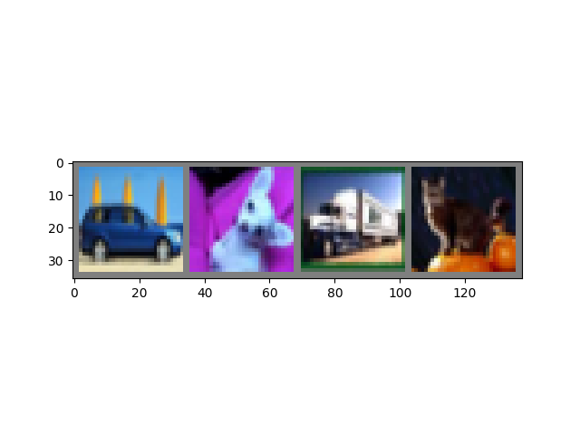
You can see that they are pretty blurry. They are:
car dog truck cat
Example: PyTorch
PyTorch lets you define a neural network with some defaults:
import torch.nn as nn
import torch.nn.functional as F


class Net(nn.Module):
    def __init__(self):
        super(Net, self).__init__()
        self.conv1 = nn.Conv2d(3, 6, 5)
        self.pool = nn.MaxPool2d(2, 2)
        self.conv2 = nn.Conv2d(6, 16, 5)
        self.fc1 = nn.Linear(16 * 5 * 5, 120)
        self.fc2 = nn.Linear(120, 84)
        self.fc3 = nn.Linear(84, 10)

    def forward(self, x):
        x = self.pool(F.relu(self.conv1(x)))
        x = self.pool(F.relu(self.conv2(x)))
        x = x.view(-1, 16 * 5 * 5)
        x = F.relu(self.fc1(x))
        x = F.relu(self.fc2(x))
        x = self.fc3(x)
        return x


net = Net()
Example: PyTorch
import torch.optim as optim

criterion = nn.CrossEntropyLoss()
optimizer = optim.SGD(net.parameters(), lr=0.001, momentum=0.9)
We can also define a loss and Sigmoid function, as we saw before:
Example: PyTorch
Now we just loop over the data and inputs, and we're training!
for epoch in range(2):  # loop over the dataset multiple times

    running_loss = 0.0
    for i, data in enumerate(trainloader, 0):
        # get the inputs; data is a list of [inputs, labels]
        inputs, labels = data

        # zero the parameter gradients
        optimizer.zero_grad()

        # forward + backward + optimize
        outputs = net(inputs)
        loss = criterion(outputs, labels)
        loss.backward()
        optimizer.step()

        # print statistics
        running_loss += loss.item()
        if i % 2000 == 1999:    # print every 2000 mini-batches
            print('[%d, %5d] loss: %.3f' %
                  (epoch + 1, i + 1, running_loss / 2000))
            running_loss = 0.0

print('Finished Training')
This was a simple, 2-iteration loop (on line 1)
Example: PyTorch
We can save the data:
PATH = './cifar_net.pth'
torch.save(net.state_dict(), PATH)- And now we can test it to see if the network has learnt anything at all.
- We will check this by predicting the class label that the neural network outputs, and checking it against the ground-truth. If the prediction is correct, we add the sample to the list of correct predictions.
- We can display an image from the test set to get familiar:
dataiter = iter(testloader)
images, labels = dataiter.next()

# print images
imshow(torchvision.utils.make_grid(images))
print('GroundTruth: ', ' '.join('%5s' % classes[labels[j]] for j in range(4)))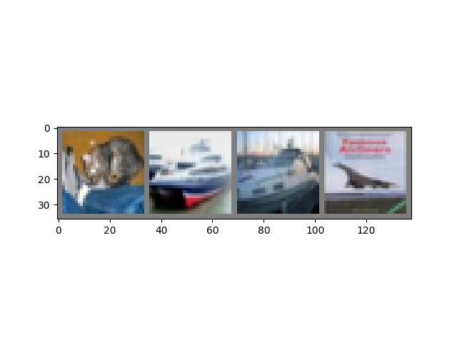
GroundTruth:
cat ship ship plane
Example: PyTorch
We can load back the data and then see how our model does:
net = Net()
net.load_state_dict(torch.load(PATH))

outputs = net(images)

_, predicted = torch.max(outputs, 1)

print('Predicted: ', ' '.join('%5s' % classes[predicted[j]]
for j in range(4)))- The higher the energy for a class, the more the network thinks that the image is of the particular class. So, we get the index of the highest energy.
- Predicted: cat car plane plane
- It got 2/4 -- not amazing, but okay all things considered.
Example: PyTorch
We can look at how the network behaves on the whole dataset:
correct = 0
total = 0
with torch.no_grad():
    for data in testloader:
        images, labels = data
        outputs = net(images)
        _, predicted = torch.max(outputs.data, 1)
        total += labels.size(0)
        correct += (predicted == labels).sum().item()

print('Accuracy of the network on the 10000 test images: %d %%' % (
100 * correct / total))- Output:
Accuracy of the network on the 10000 test images: 53 %- This is better than chance, which would have been 10%
Example: PyTorch
We can see which categories did well:
class_correct = list(0. for i in range(10))
class_total = list(0. for i in range(10))
with torch.no_grad():
    for data in testloader:
        images, labels = data
        outputs = net(images)
        _, predicted = torch.max(outputs, 1)
        c = (predicted == labels).squeeze()
        for i in range(4):
            label = labels[i]
            class_correct[label] += c[i].item()
            class_total[label] += 1


for i in range(10):
    print('Accuracy of %5s : %2d %%' % (
classes[i], 100 * class_correct[i] / class_total[i]))- Output:
GroundTruth:    cat  ship  ship plane
Predicted:    dog  ship  ship  ship
Accuracy of the network on the 10000 test images: 55 %
Accuracy of plane : 67 %
Accuracy of   car : 72 %
Accuracy of  bird : 36 %
Accuracy of   cat : 18 %
Accuracy of  deer : 45 %
Accuracy of   dog : 60 %
Accuracy of  frog : 64 %
Accuracy of horse : 62 %
Accuracy of  ship : 65 %
Accuracy of truck : 65 %
- How could we improve? More loops!
Example: PyTorch
2 loops:
GroundTruth:    cat  ship  ship plane
Predicted:    cat  ship plane plane
Accuracy of the network on the
            10000 test images: 61 %
Accuracy of plane : 66 %
Accuracy of   car : 77 %
Accuracy of  bird : 47 %
Accuracy of   cat : 33 %
Accuracy of  deer : 63 %
Accuracy of   dog : 53 %
Accuracy of  frog : 71 %
Accuracy of horse : 54 %
Accuracy of  ship : 74 %
Accuracy of truck : 72 %
GroundTruth: cat ship ship plane
Predicted: dog ship ship ship
Accuracy of the network on the
10000 test images: 55 %
Accuracy of plane : 67 %
Accuracy of car : 72 %
Accuracy of bird : 36 %
Accuracy of cat : 18 %
Accuracy of deer : 45 %
Accuracy of dog : 60 %
Accuracy of frog : 64 %
Accuracy of horse : 62 %
Accuracy of ship : 65 %
Accuracy of truck : 65 %- The model is getting better!
Using Python for Artificial Intelligence
By Chris Gregg


