Intervention

Analysis
I. Theory
II. R Example
III. Applications

Breif HISTORY & Theory
- Intervention analysis, sometimes called interrupted time-series analysis, estimates the effect of an external or exogenous intervention on a time-series.
- Interrupted time-series is a special kind of time series in which we know the specific point in the series at which an intervention occurred.
- Typically conducted with the Box & Jenkins ARIMA framework, using the methods outlined by Box & Tiao in 1965.
- Other methods such as segmented regression may be used.
- Developed in the 1970’s out of the long time practice of pre and post treatment testing in scientific experiments.
- Causal hypothesis is that observations after treatment will have a different level or slope from those before intervention – the interruption
-
Forces other than the intervention under investigation influenced the dependent variable
-
Could add a no-treatment time series from a control group
-
Use qualitative or quantitative means to examine plausible effect-causing events
-
Instrumentation – how was data collected/recorded
-
Selection – did the composition of the experimental group change at the time of intervention?
-
Poorly specified intervention point; diffusion
Threats of validity:
-
Choice of outcome – usually have only routinely collected data
-
Power, violated test assumptions, unreliability of measurements, reactivity etc.
Four
basic types of interventions
Step
Delayed Step
pulse
Decayed Pulse


ARIMA
model without intervention
Y_t - \bar Y = \frac{\theta(B)}{\phi(B)}e_t
Yt−Y¯=ϕ(B)θ(B)et
ARIMA
model with intervention
Y_t - \bar Y = z_t + \frac{\theta(B)}{\phi(B)}e_t
Yt−Y¯=zt+ϕ(B)θ(B)et
where is the amount of change at time that is attributed to
the intervention. By definition is 0 before .
z_t
zt
t
t
z_t
zt
t
t
PATTERN 1:
Permanent constant change to the mean level: An amount has been added (or subtracted) to each value after time T.
Constant change after time T may be written simply as:
z_t = \delta_0I_t
zt=δ0It
where
I_t = 0
It=0
t < T
t<T
when
I_t = 1
It=1
t \geq T
t≥T
Overall intervention model:
when
Y_t - \bar Y = \delta_0 I_t + \frac{\theta(B)}{\phi(B)}e_t
Yt−Y¯=δ0It+ϕ(B)θ(B)et
Step
PATTERN 2:
Brief constant change to the mean level: There may be a temporary change for one or more periods, after which there is no effect of the intervention.

Brief change after time T may be written simply as:
z_t = \delta_0(I_t-I'_t)
zt=δ0(It−It′)
where
I'_t = 0
It′=0
t < T+d
t<T+d
when
I'_t = 1
It′=1
Overall intervention model:
when
Y_t - \bar Y = \delta_0 (I_t-I'_t) + \frac{\theta(B)}{\phi(B)}e_t
Yt−Y¯=δ0(It−It′)+ϕ(B)θ(B)et
t \geq T+d
t≥T+d
pulse
PATTERN 3:
Gradually increasing/decreasing which levels off.
Change after time T may be written simply as:
z_t = \frac{\delta_0}{1-w_1B}I_t
zt=1−w1Bδ0It
Overall intervention model:
Y_t - \bar Y = \frac{\delta_0}{1-w_1B}I_t + \frac{\theta(B)}{\phi(B)}e_t
Yt−Y¯=1−w1Bδ0It+ϕ(B)θ(B)et
where
|w_1| < 1
∣w1∣<1
Delayed Step
PATTERN 4:
Immediate change which returns to original level.
Change after time T may be written simply as:
z_t = \frac{\delta_0}{1-w_1B}P_t
zt=1−w1Bδ0Pt
Overall intervention model:
Y_t - \bar Y = \frac{\delta_0}{1-w_1B}P_t + \frac{\theta(B)}{\phi(B)}e_t
Yt−Y¯=1−w1Bδ0Pt+ϕ(B)θ(B)et
where
P_t = 1
Pt=1
Decayed PULSE
when
t = T
t=T
USEFUL in explaining the effect of an intervention and so they help improve forecast accuracy after an intervention.
LIMITED VALUE in forecasting the effect of an intervention before it occurs as we cannot estimate (because of the lack of data) the parameters of the intervention model.
Intervention Model
R
in
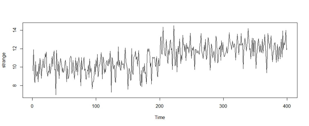
Seems like a series that is generally stationary, but shifts level around t=200.
Looks like two separate leveled series before and after t=200.
Examine separately at the parts before and after the level shift. There are in total 400 time-points. Select the first 190 and the last 190 observations.
First 190 data points
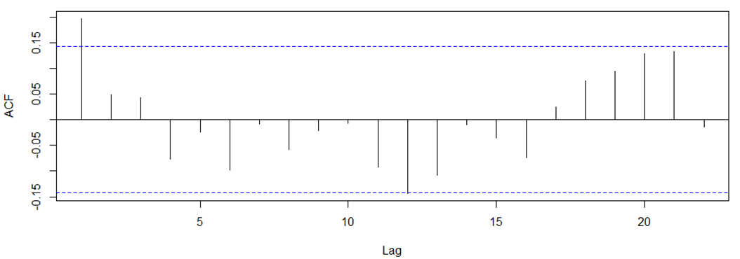
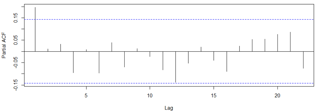
Stationary data
AR(1)?
MA(1)?
ARMA(1,0,1)?
LAST 190 data points
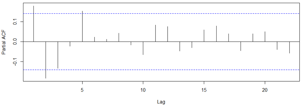
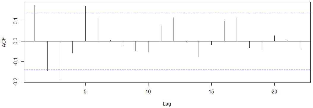
Stationary data
ARMA(1,0,1)!
A STEP function
Seems to be a permanent, immediate, and constant change in level at t = 200

Y_t=\bar Y+\delta_0 I_t+\frac{1-\theta_1 B}{1-\phi_1 B}e_t
Yt=Y¯+δ0It+1−ϕ1B1−θ1Bet
Let:
Our model is:
ARIMA(1,0,1)
strange.model <-arimax(strange,order=c(1,0,1),
                       xtransf=data.frame(step200=1*(seq(strange)>=200)),
                       transfer=list(c(0,0)))
- The arimax command works like the arima command, but allows inclusion of co-variates.
- The argument xtransf is followed by a data frame in which each column correspond to a co-variate time series (same number of observations as ).
Y_t
Yt
To model the intervention model using TSA library
- Data frame: 1*(seq(strange)>=200).
- Transfer is followed by a list comprising one two-dimensional vector for each co-variate specified by xtransf.
strange.model <-arimax(strange,order=c(1,0,1),
                       xtransf=data.frame(step200=1*(seq(strange)>=200)),
                       transfer=list(c(0,0)))
- list(c(0,0)) implies that the co-variate shall be included as it stands (no lagging, no filtering).
- c(r,s) where both r and s are > 0 will enter the term
\delta_0 \frac{1-w_1B-w_2B^2...-w_sB^s}{1-\sigma_1B-\sigma_2B^2...-\sigma_rB^r}I_t
δ01−σ1B−σ2B2...−σrBr1−w1B−w2B2...−wsBsIt
- c(0,0) gives
\delta_0I_t
δ0It
print(strange.model)Series: strange
ARIMA(1,0,1) with non-zero mean
Coefficients:
ar1 ma1 intercept step200-MA0
0.9824 -1.0000 10.0026 1.9958
s.e. 0.0111 0.0064 0.0350 0.0606
sigma^2 estimated as 0.9826: log likelihood=-564.82
AIC=1137.64 AICc=1137.79 BIC=1157.6
Thus, our model is:
Y_t=10.0026+1.9958I_t+\frac{1+ B}{1-0.9824 B}e_t
Yt=10.0026+1.9958It+1−0.9824B1+Bet
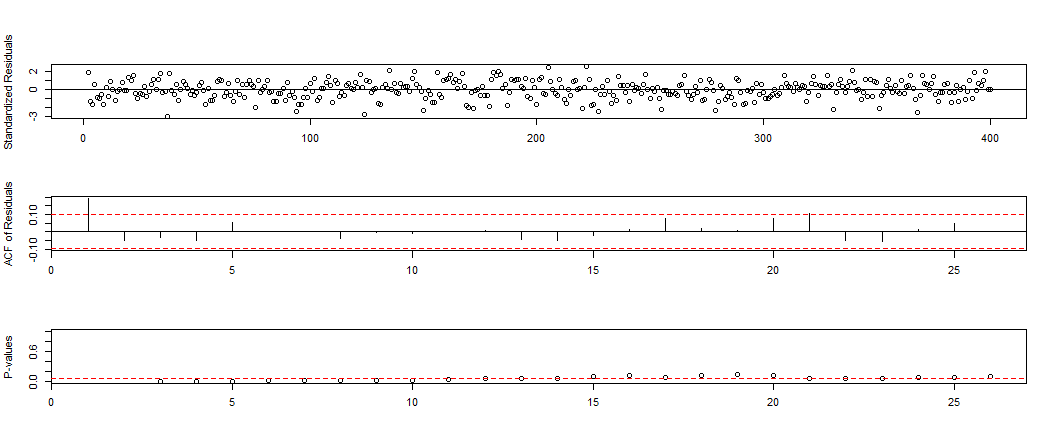
Seems to be some auto-correlation left in the residuals.
Try an ARMA(1,0,2)
strange.model2 <-arimax(strange,order=c(1,0,2),
                 xtransf=data.frame(step200=1*(seq(strange)>=200)),
                 transfer=list(c(0,0)))
Series: strange
ARIMA(1,0,2) with non-zero mean

Coefficients:
         ar1      ma1      ma2  intercept  step200-MA0
      0.9730  -0.7781  -0.2219    10.0012       1.9972
s.e.  0.0133   0.0525   0.0521     0.0317       0.0557

sigma^2 estimated as 0.9406:  log likelihood=-556.28
AIC=1122.56   AICc=1122.77   BIC=1146.5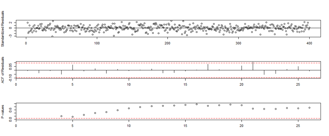
Y_t=10.0012+1.9972I_t+\frac{1+ B}{1-0.9730 B}e_t
Yt=10.0012+1.9972It+1−0.9730B1+Bet
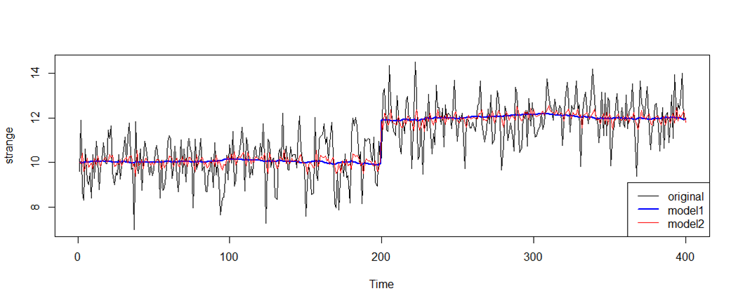
plot(y=strange,x=seq(strange),type="l",xlab="Time")
lines(y=fitted(strange.model),x=seq(strange),col="blue", lwd=2)
lines(y=fitted(strange.model2),x=seq(strange),col="red", lwd=1)
legend("bottomright",legend=c("original","model1","model2"),
       col=c("black","blue","red"),lty=1,lwd=c(1,2,1))
Intervention Analysis

Analytic
ForeCast
Intervention Analysis
Changes to a procedure, or law, or policy

Crisis, Man-made/ natural disasters

Applications
- stock prices

Chinese stock prices
Source: ARIMA Modeling With Intervention to Forecast and Analyze Chinese Stock Prices
- The results indicate that the World Financial Crisis in 2008 had an alarming intervention effect clearly felt by the financial industry in China.
- Use of intervention analysis is very useful in explaining the dynamics of the impact of serious interruptions in an economy and the changes in the time series of a price index in a precise and detailed manner.
- demand forecast

Inbound Tourism demand
Source: Intervention analysis of inbound tourism: A case study of Taiwan
- Taiwan's inbound tourism was affected by the September 21st Earthquake in 1999 and the Severe Acute Respiratory Syndrome (SARS) outbreak in 2003, one of the mega earthquakes in the 20th century and most catastrophic health hazard in the past hundred years in Taiwan, respectively.
- The inbound tourism was more heavily influenced by the SARS epidemic and recovered from the SARS shadow was greater compared with the recovery after the September 21st Earthquake.
Applications
- others

Crime rates
Source: Intervention time series analysis of crime rates: the impact of sentence reforms in Virginia
- Proposed models for analysing the effects of parole abolition and sentence reform in Virginia clearly favour ARIMA or structural time series approaches to modelling intervention. Results using regression approaches are biased and the measured effects are not reliable because of the serially correlated errors.
Applications
- others
sales vs promotion
Applications
car accidents vs speed limit
Pollution level vs opening of freeway

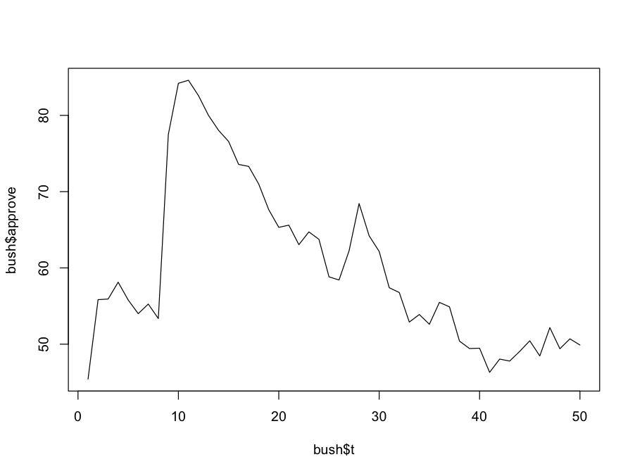
President Bush's approval ratings
A fun example
Source: R-bloggers.com
   year month  approve  t s11
1  2001     1 45.41947  1   0
2  2001     2 55.83721  2   0
3  2001     3 55.91828  3   0
4  2001     4 58.12725  4   0
5  2001     5 55.79231  5   0
.
.
.- A study by University of Georgia political science professor Jamie Monogan
- Impact of some EVENTS on Bush's approve ratings
- Data:
Decayed Pulse
Y_t - \bar Y = \frac{\delta_0}{1-w_1B}P_t + \frac{\theta(B)}{\phi(B)}e_t
Yt−Y¯=1−w1Bδ0Pt+ϕ(B)θ(B)et
#libraries
rm(list=ls())
library(foreign)
library(TSA)

setwd('/Users/wkuuser/Desktop/briefcase/R Data Sets') # mac

#load data & view series
bush <- read.dta("BUSHJOB.DTA")
names(bush)
print(bush)

plot(y=bush$approve, x=bush$t, type='l')

#identify arima process
acf(bush$approve)
pacf(bush$approve)

#estimate arima model
mod.1 <- arima(bush$approve, order=c(0,1,0))
mod.1

#diagnose arima model
acf(mod.1$residuals)
pacf(mod.1$residuals)
Box.test(mod.1$residuals)

#Looks like I(1)
#estimate intervention analysis
mod.2 <- arimax(bush$approve, order=c(0,1,0), xtransf=bush$s11, transfer=list(c(1,0)))
mod.2
summary(mod.2)

#Our parameter estimates look good, no need to drop delta or switch to a step function.

#Graph the intervention model
y.diff <- diff(bush$approve)
t.diff <- bush$t[-1]
y.pred <- 24.3741*bush$s11 + 24.3741*(.9639^(bush$t-9))*as.numeric(bush$t>9)
y.pred <- y.pred[-1]
plot(y=y.diff, x=t.diff, type='l')
lines(y=y.pred, x=t.diff, lty=2)

#suppose an AR(1) process
mod.2b <- arimax(bush$approve, order=c(1,0,0), xtransf=bush$s11, transfer=list(c(1,0)));
mod.2b
y.pred <- 58.2875 + 23.6921*bush$s11 + 23.2921*(.8915^(bush$t-9))*as.numeric(bush$t>9)
plot(y=bush$approve, x=bush$t, type='l')
lines(y=y.pred, x=bush$t, lty=2)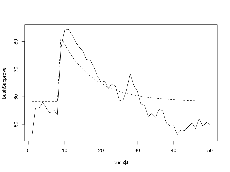
Observation 10 represents October 2001, post 9/11/2011.
A DRASTIC shift in the series, that slowly decays and eventually returns to previous levels.
2001/10
"But Mr. Bush enjoyed a high approval rating of 90 percent -- the highest of any president -- following the Sept. 11 attacks in 2001. "
"President Bush [left] office as one of the most unpopular departing presidents in history, according to a new CBS News/New York Times poll showing Mr. Bush's final approval rating at 22 percent."


No questions please!
Enjoy your break!
Intervention Analysis
By tony g


