DESPOT/DESPOT-\(\alpha\)
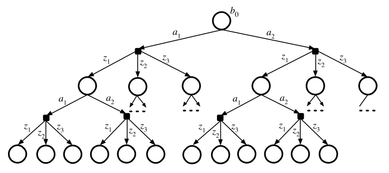
Standard Belief Tree
\(\mathcal{O}(|A|^DC^D) \)(|A|^D||Z|^D)
DESPOT
\(\mathcal{O}(K|A|^D)\)
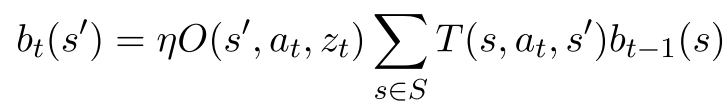
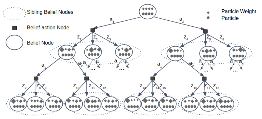
DEterminized Sparse Partially Observable Tree
Sparse: Create subset of possible state trajectories from belief tree via scenarios
Determinized: Scenarios are randomly sampled state trajectories using a deterministic simulative model
Text
\text{Scenario: } (s_0, \phi_1, \phi_2, \dots), \quad s_0 \sim b_0, \phi_i \sim \mathcal{U}[0,1]
\quad \rightarrow \quad
s',z = G(s, a, \phi)
Determinization
Purpose: Don't want to attribute reward gains or losses due to process noise to the value inherent to a belief state.
Consequence: Possible Overfitting
\hat{V}_{\pi}(b)=\sum_{\phi \in \Phi_{b}} \frac{V_{\pi, \phi}}{\left|\Phi_{b}\right|}
Empirical policy belief value
\hat{\pi}^{*} = \max_{\pi \in \Pi_{\mathcal{D}}}\left\{\hat{V}_\pi(b_0)\right\} \quad \rightarrow \quad
\hat{\pi}^{*} = \max_{\pi \in \Pi_{\mathcal{D}}}\left\{\hat{V}_\pi(b_0) - \lambda |\pi|\right\}
Generalizing to any node in the constructed tree, define regularized, weighted, discounted utility (RWDU) as:
\nu_{\pi}(b)=\frac{\left|\Phi_{b}\right|}{K} \gamma^{\Delta(b)} \hat{V}_{\pi_{b}}(b)-\lambda\left|\pi_{b}\right|
Regularize Reward
Belief Node Backup
Start at leaf belief nodes
Move through internal belief nodes
\nu^{*}(b)=\max \left\{\frac{\left|\Phi_{b}\right|}{K} \gamma^{\Delta(b)} \hat{V}_{\pi_{0}}(b), \max _{a \in A}\left\{\rho(b, a)+\sum_{z \in Z_{b, a}} \nu^{*}(\tau(b, a, z))\right\}\right\}
a^* = \argmax _{a \in \mathcal{A}}\left\{\rho(b_0, a)+\sum_{z \in Z_{b_0, a}} \nu^{*}(\tau(b_0, a, z))\right\}
\nu^{*}(b)=\frac{\left|\Phi_{b}\right|}{K} \gamma^{\Delta(b)} \hat{V}_{\pi_{0}}(b)
Evaluate best action at root belief node
\rho(b, a)=\frac{1}{K} \sum_{\phi \in \Phi_{b}} \gamma^{\Delta(b)} R\left(s_{\phi}, a\right)-\lambda
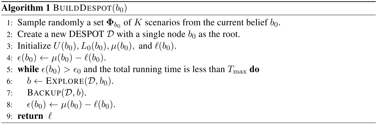
ARDESPOT
(Anytime Regularized DESPOT)
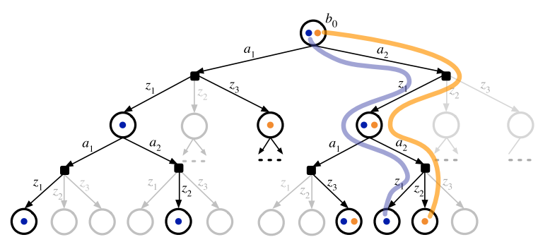
Construct tree incrementally with belief value bounds heuristics
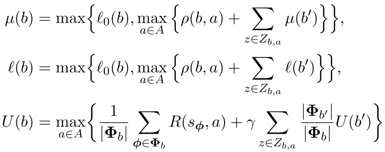
\(l(b), \mu(b)\) : lower and upper bounds of optimal RWDU at belief node \(b\) \(\rightarrow l(b) \le \nu^*(b) \le \mu(b)\)
\( L_0(b), U(b)\) : lower and upper bounds of non-regularized belief value \(\rightarrow L_0(b) \le \hat{V}^*(b) \le U(b)\)
l_0(b') = \nu_{\pi_0}(b') = \frac{|\mathbf{\Phi_{b'}}|}{K}\gamma^{\Delta(b')}L_0(b')
\mu_0(b') = \max\left\{l_0(b'),\frac{|\mathbf{\Phi_{b'}}|}{K}\gamma^{\Delta(b')}U_0(b') - \lambda\right\}
L_0(b) = \hat{V}_{\pi}(b)=\sum_{\phi \in \Phi_{b}} \frac{V_{\pi, \phi}}{\left|\Phi_{b}\right|}
a^{*}=\underset{a \in A}{\arg \max }
\left\{\mu(b, a)\right\}=\underset{a \in A}{\arg \max }\left\{\rho(b, a)+\sum_{z \in Z_{b, a}} \mu\left(b^{\prime}\right)\right\}
z^{*}=\underset{z \in Z_{b, a^{*}}}{\arg \max } \left\{ E\left(b^{\prime}\right) \right\}
=\underset{z \in Z_{b, a^{*}}}{\arg \max }\left\{\epsilon\left(b^{\prime}\right)-\frac{\left|\Phi_{b^{\prime}}\right|}{K} \cdot \xi \epsilon\left(b_{0}\right)\right\}
\(\xi\) : Tuning parameter - Desired RWDU bounds contraction rate at root node \(b_0\)
Cease exploration once \(E(b') \le 0 \). Exploration beyond this point yields minimal RWDU bounds contraction
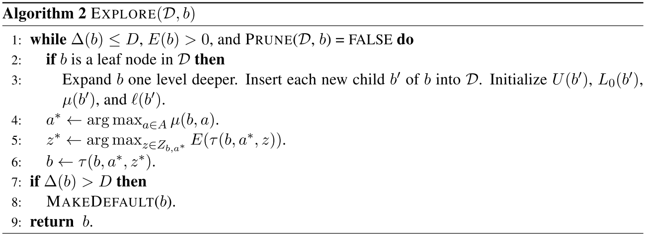
Pruning
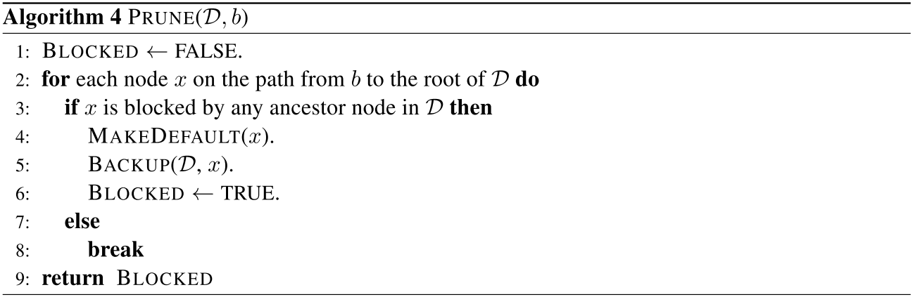
\frac{\left|\Phi_{b^{\prime}}\right|}{K} \gamma^{\Delta\left(b^{\prime}\right)}\left(U\left(b^{\prime}\right)-L_{0}\left(b^{\prime}\right)\right) \leq \lambda \cdot \ell\left(b^{\prime}, b\right)
Blocked if
Backup
DESPOT-\(\alpha\)
DESPOT with \(\alpha\)-vector update
w_{\tau(b, a, z)}\left(s^{\prime}\right)=\frac{p\left(z \mid s^{\prime}, a\right) \sum_{s \in \Phi_{b}} p\left(s^{\prime} \mid s, a\right) w_{b}(s)}{p(z \mid b, a)}
b(s) = w_b(s)
Q(b,a) = \sum_{s\in\Phi_b}w_b(s)R(s,a) + \gamma\sum_{z\in C_{b,a}}p(z|b,a)V(\tau(b,a,z))
Belief in state determined by weight of representative particle
- Using \(C \le K\) scenarios at each belief-action node to generate observation branches
- Re-weighting all particles for each new belief node is computationally costly relative to DESPOT
- Save computation time using parallelizable \(\alpha\)-vectors on sibling nodes
- Sibling nodes share same scenarios with same states just different beliefs over these states
- Assume sibling beliefs are similar in terms of conditional plan that maximizes their values
- Holds for larger observation spaces
\underline{V}_{n}(b)=\sum_{s \in \Phi_{b}} w_{b}(s) \alpha_{n, b}(s) = \vec{\alpha}_{n, b}^T\vec{w}_b
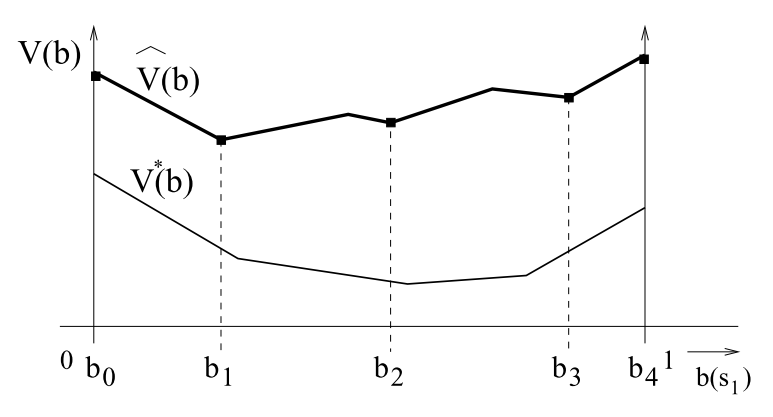
Upper bounds maintained with sawtooth approximation
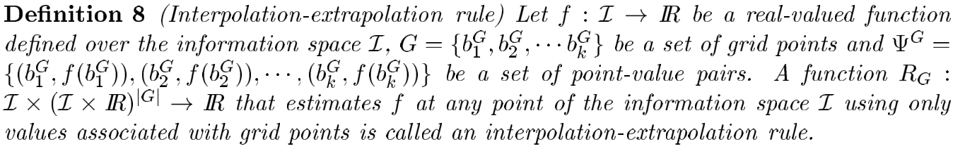
\varphi_{i+1}\left(b_{j}^{G}\right)=\left(H \widehat{V}_{i}\right)\left(b_{j}^{G}\right)=\max _{a \in A}\left\{\rho(b, a)+\gamma \sum_{o \in \Theta} P(o \mid b, a) \widehat{V}_{i}\left(\tau\left(b_{j}^{G}, o, a\right)\right)\right\}
\widehat{V}_{i}(b)=\min _{b^{\prime} \in G} \widehat{V}_{i}^{b^{\prime}}(b)
Choose set of grid points to be an arbitrary grid point \(b' \in G\) and \(|S|-1\) extreme points of the belief simplex
\alpha_{0, b}(s)=\alpha_{b_{0}, \zeta(b)}^{d e f}(s)=\sum_{t=d}^{\infty} \gamma^{d} R\left(s_{t}, \pi_{d e f}\left(b_{0}, \zeta(b)\right) \mid s_{d}=s\right) \\
\zeta(b) = a_0,a_1,\dots a_{d-1}
Leaf Node
Internal Nodes
\underline{V}_{n+1}(b)=\max _{a \in A}\left\{\sum_{s \in \Phi_{b}} w_{b}(s) R(s, a)+\gamma \sum_{z \in C_{b}, a} p(z \mid b, a) \underline{V}_{n}(\tau(b, a, z))\right\}
\underline{V}_{n+1}(b)=\sum_{s \in \Phi_{b}} w_{b}(s)\left(\alpha_{n+1, b}(s)\right) \text { s.t. } \alpha_{n+1, b}(s)=\alpha_{n+1, b}^{a^{*}}(s)
\alpha_{n+1, b}^{a}(s)=R(s, a)+\gamma \sum_{z \in C_{b, a}} p\left(z \mid s_{+}, a\right) \alpha_{n, \tau(b, a, z)}\left(s_{+}\right)
a^{*}=\underset{a \in A}{\arg \max }\left\{\sum_{s \in \Phi_{b}} w_{b}(s) \alpha_{n+1, b}^{a}(s)\right\}
Text
DESPOT-(alpha)
By Tyler Becker


