Binary classification
Classification
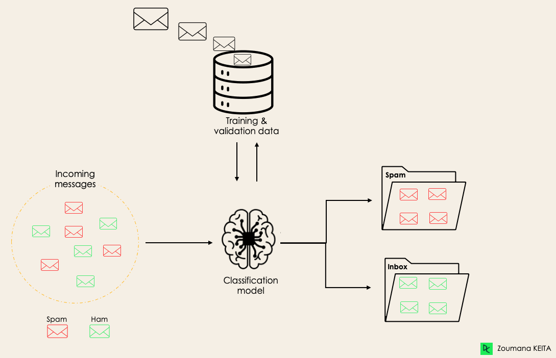
Identify and separate observations into distinct categories.
Examples: tag emails as spam, diagnose a particular disease in a patient, identify defective products in a factory line, discard background events in physics analysis, etc...
Classification
Any algorithm or procedure that maps a set of inputs into a discrete value is called a "Classifier"
In general this will be some kind of function of N variables (or features) grouping events into classes, according to the values of the associated variables.
Binary classification: only two categories/classes are considered
Relevant concepts
Confusion matrix:
- Summary of the probability of correct and incorrect predictions
| S (predicted) | B (predicted) | |
| S (real) | True positives | False negatives |
| B (real) | False positives | True negatives |
Type I Error
Type II Error
Relevant concepts
Confusion matrix:
- Summary of the probability of correct and incorrect predictions
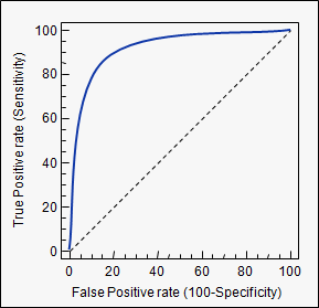
Receiver Operating Characteristic (ROC)
- Only valid for binary classifiers
- Shows performance of the classifier for all working points
- Can be summarized in a single value (Area Under Curve - AUC) to represent classification power
The dataset
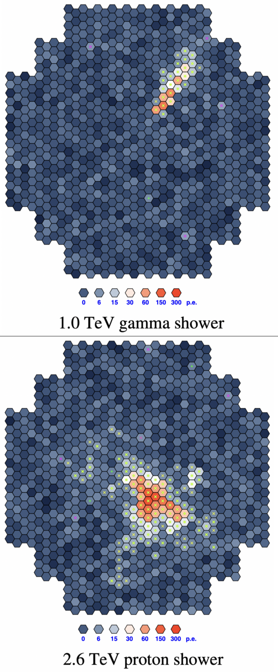
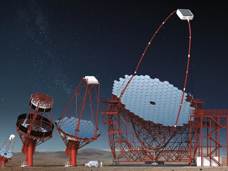
Simulation from the CTA experiment
Goal: reject showers caused by hadrons, while keeping showers from gamma rays
10 features (variables)
We will try two methods
- Likelihood ratio
- Boosted Decision Trees (BDT)
The dataset
You will be given a ROOT file with two TTree objects inside (one for Signal events, one for Background events), each having 10 Branches
❯ root -l magic04.root
root [0]
Attaching file magic04.root as _file0...
(TFile *) 0x555bf47811c0
root [1] .ls
TFile**		magic04.root
 TFile*		magic04.root
  KEY: TTree	Signal;1
  KEY: TTree	Background;1
root [2] Signal->Print()
******************************************************************************
*Tree    :Signal    :                                                        *
*Entries :    12332 : Total =          501716 bytes  File  Size =     395259 *
*        :          : Tree compression factor =   1.00                       *
******************************************************************************
*Br    0 :fLength   : fLength/F                                              *
*Entries :    12332 : Total  Size=      50149 bytes  All baskets in memory   *
*Baskets :        1 : Basket Size=      32000 bytes  Compression=   1.00     *
*............................................................................*
*Br    1 :fWidth    : fWidth/F                                               *
*Entries :    12332 : Total  Size=      50141 bytes  All baskets in memory   *
*Baskets :        1 : Basket Size=      32000 bytes  Compression=   1.00     *
*............................................................................*
*Br    2 :fSize     : fSize/F                                                *
*Entries :    12332 : Total  Size=      50133 bytes  All baskets in memory   *
*Baskets :        1 : Basket Size=      32000 bytes  Compression=   1.00     *
*............................................................................*
*Br    3 :fConc     : fConc/F                                                *
*Entries :    12332 : Total  Size=      50133 bytes  All baskets in memory   *
*Baskets :        1 : Basket Size=      32000 bytes  Compression=   1.00     *
*............................................................................*
*Br    4 :fConc1    : fConc1/F                                               *
*Entries :    12332 : Total  Size=      50141 bytes  All baskets in memory   *
*Baskets :        1 : Basket Size=      32000 bytes  Compression=   1.00     *
*............................................................................*
*Br    5 :fAsym     : fAsym/F                                                *
*Entries :    12332 : Total  Size=      50133 bytes  All baskets in memory   *
*Baskets :        1 : Basket Size=      32000 bytes  Compression=   1.00     *
*............................................................................*
*Br    6 :fM3Long   : fM3Long/F                                              *
*Entries :    12332 : Total  Size=      50149 bytes  All baskets in memory   *
*Baskets :        1 : Basket Size=      32000 bytes  Compression=   1.00     *
*............................................................................*
*Br    7 :fM3Trans  : fM3Trans/F                                             *
*Entries :    12332 : Total  Size=      50157 bytes  All baskets in memory   *
*Baskets :        1 : Basket Size=      32000 bytes  Compression=   1.00     *
*............................................................................*
*Br    8 :fAlpha    : fAlpha/F                                               *
*Entries :    12332 : Total  Size=      50141 bytes  All baskets in memory   *
*Baskets :        1 : Basket Size=      32000 bytes  Compression=   1.00     *
*............................................................................*
*Br    9 :fDist     : fDist/F                                                *
*Entries :    12332 : Total  Size=      50133 bytes  All baskets in memory   *
*Baskets :        1 : Basket Size=      32000 bytes  Compression=   1.00     *
*............................................................................*
Lesson 01
We will begin with an "exploratory" exercise.
Lesson 01
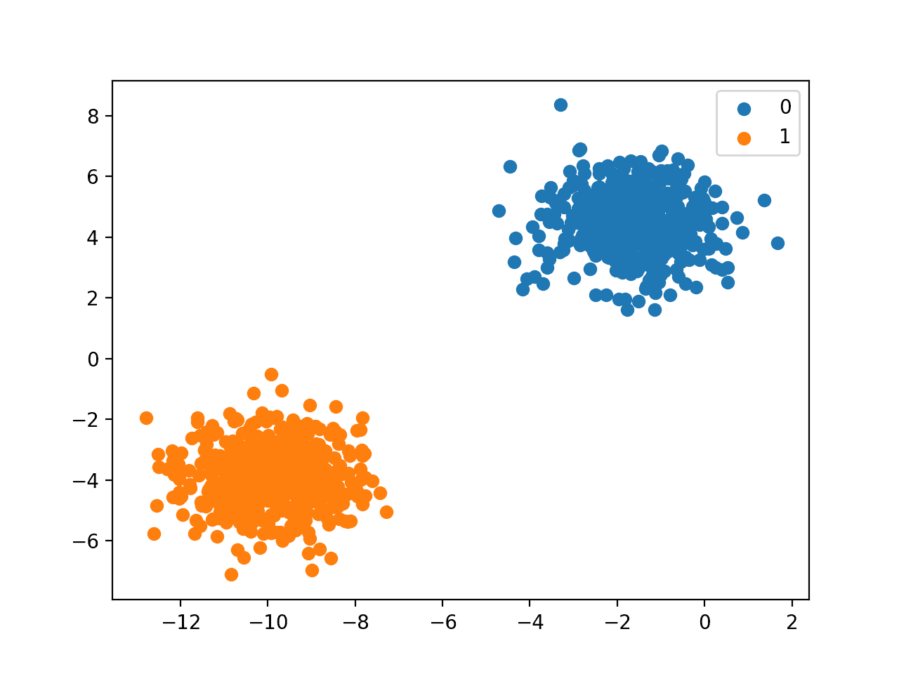
Before attempting to build a classifier it is always a good idea to visualize the dataset and get a feeling of how different the classes are, among the features of the dataset.
Refreshing the basics
Main goals:
- Get the fundamentals of classification
- Compare different classifiers
- Get familiar with C++ and ROOT
(this will mean writing and running most of the code yourself)
You will find the data at ~vformato/2023/data/magic04.root on the course VM
Refreshing the basics
Opening a file
- If you just need to read from the file then TFile::Open() is the easiest way
- It returns a TFile*, you can either call delete on it when you're done, or TFile::Close.
If you don't sometimes can lead to strange crashes
TFile* my_file = TFile::Open("filename.root");

// ...

my_file->Close();
Refreshing the basics
Getting objects from files
- Prefer using TFile::Get<T> rather than TFile::GetObject
(you can avoid a cast, just make sure you use the right type between <>) - You get a raw pointer back, but it will be null if the object is not on file.
(You might have to check that manually) - Objects from files go out of scope when the file is closed.
HUGE SOURCE OF BUGS
TH1D* histo_from_file = my_file->Get<TH1D>("histo");
// Older alternative:
// TH1D* histo_from_file = (TH1D*) my_file->GetObject("histo");

if (!histo_from_file){
  std::cerr << "Could not find histo on file!\n";
}
Refreshing the basics
Looping over a TTree:
- After retrieving the tree from file you need a "placeholder" in memory
- You tell the tree where the placeholder for each variable is with SetBranchAddress
- Loop over all the entries in the tree and call GetEntry for each of them. Now the placeholders will contain the value of the tree variable for that particular entry.
TTree* my_tree = my_file->Get<TTree>("tree");

int intVar;
float floatVar;

my_tree->SetBranchAddress("intVar", &intVar);
my_tree->SetBranchAddress("floatVar", &floatVar);

size_t n_events = my_tree->GetEntries();
for (size_t iev = 0; iev < n_events; ++iev) {
  my_tree->GetEntry(iev);

  // now you can use intVar and/or floatVar
}
Creating objects
ROOT tutorials and most people will teach to use new to create objects such as histograms and trees.
This is because the ROOT interpreter has some internal mechanism of ownership and memory management but in general it's not considered a good practice.
However, if you follow "good practice" you'll have problems due to how ROOT expects objects to live.
TTree* my_tree = my_file->Get<TTree>("tree");

int intVar;
float floatVar;

my_tree->SetBranchAddress("intVar", &intVar);
my_tree->SetBranchAddress("floatVar", &floatVar);

TH1D* my_histo_i = new TH1D("histo_i", "Title;Xlabel;Ylabel", 100, 0, 100);
TH1D* my_histo_f = new TH1D("histo_f", "Title;Xlabel;Ylabel", 100, 0, 100);

size_t n_events = my_tree->GetEntries();
for (size_t iev = 0; iev < n_events; ++iev) {
  my_tree->GetEntry(iev);

  my_histo_i->Fill(intVar);
  my_histo_f->Fill(floatVar);
}
Drawing objects
Histograms and graphs can be drawn on screen using the Draw() method.
It is often useful to do it on a pre-created TCanvas.
This allows you to specify the size of the window, divide the canvas into multiple sub-plots, and even print it as a png/pdf...
// ...
TH1D* my_histo1 = new TH1D("histo1", "Title;Xlabel;Ylabel", 100, 0, 100);
TH1D* my_histo2 = new TH1D("histo2", "Title;Xlabel;Ylabel", 100, 0, 100);

size_t n_events = my_tree->GetEntries();
for (size_t iev = 0; iev < n_events; ++iev) {
  //...
}

TCanvas* my_canvas = new TCanvas("canvas", "My Title", 0, 0, 1024, 600);
my_canvas->Divide(2, 1); // 2 sub-canvas in one line

my_canvas->cd(1);
my_histo1->Draw();

my_canvas->cd(2);
my_histo2->Draw();

my_canvas->Print("my_plot.png");
Goal for today
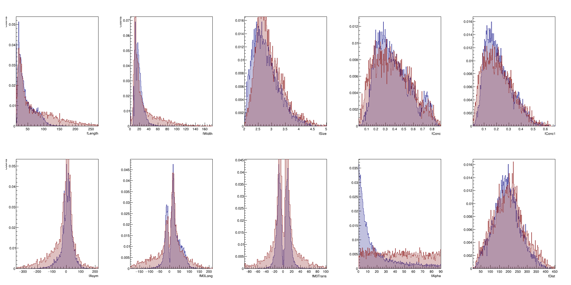
As a first step try to visualize the distribution of each feature by comparing signal vs background.
You want to get a feeling of which variable is more powerful and which ones might need some normalization / scaling / transformation.
This will still be very useful since it's basically the first step in order to build a likelihood function.
Goal for today
As a first step try to visualize the distribution of each feature by comparing signal vs background.
You want to get a feeling of which variable is more powerful and which ones might need some normalization / scaling / transformation.
This will still be very useful since it's basically the first step in order to build a likelihood function.
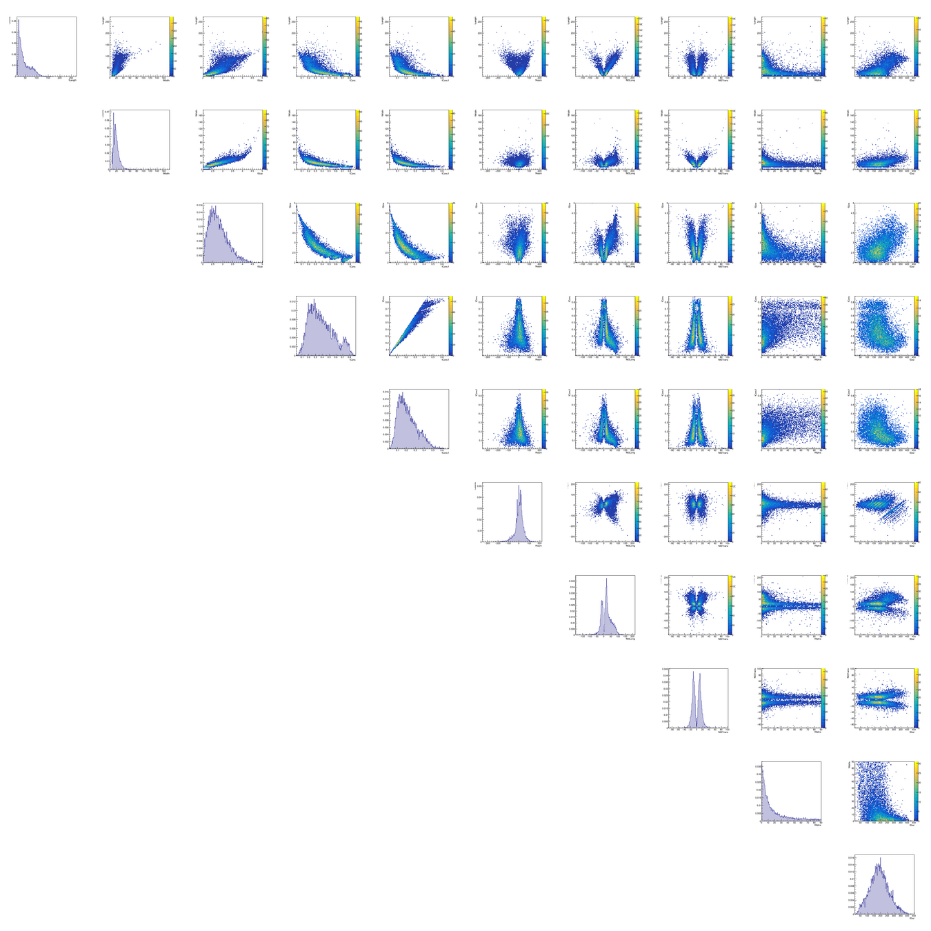
(Bonus points if you manage to do also correlation plots)
Lesson 02/03
Now we will build a Maximum Likelihood estimator
What is a Likelihood
The Likelihood function is defined as the joint probability for observing the simultaneous realization of \(N\) random variables, as a function of their p.d.f. parameters
$$\mathcal L(\mathbf \theta) \equiv \prod_{i=1}^N P (\mathbf x_i; \mathbf \theta) $$
Usually you'd want to use this to find the set of parameters that maximise this function and use it as an estimator for some physical observable(s)
$$\hat \theta = \argmax_\theta \mathcal L (\theta)$$
But it can also be used as a binary (or multi-class) classifier
Under the assumption that all observations are i.i.d
Likelihood ratio classifier
Suppose we have a set of \(N\) features (i.e. variables) \(\mathbf x\) and our observations all belong to the set of classes \( \mathcal Y = \{+1, -1\} \) (i.e. signal and background)
Now let us define as \(f_{+1}\) and \(f_{-1}\) as the joint p.d.f. for \(\mathbf x\) for the two classes
$$ f_{+1} (\mathbf x) = f(\mathbf x \, | \, Y = +1) \, , \, f_{-1} (\mathbf x) = f(\mathbf x \, | \, Y = -1)$$
also known as conditional probabilities
Let us now define the Likelihood ratio as
$$ \lambda = \frac {\mathcal L_{+1}}{\mathcal L_{-1}} \equiv \frac {f_{+1} (\mathbf x)}{f_{-1} (\mathbf x)} $$
and we can generally assign a class to an event if \( \lambda > k \) for a given value of \(k\) that we will choose in order to reach the desired level of accuracy (and/or purity)
log-likelihood
Now we turn our attention to the conditional probabilities
Even though it is almost always never the case, we can start by assuming all the features are independent from each other, so:
$$ \mathcal L_{\pm 1} = f_{\pm 1} (\mathbf x) =\prod_{i=1}^N P_i^{\pm 1} (x_i; \mathbf \theta) $$
and we can use the marginal p.d.f. of each feature to compute the two likelihoods.
It is usually helpful to work in term of the log-likelihood:
$$ \log \mathcal L_{\pm 1} = \sum_{i=1}^N \log P_i^{\pm 1} (x_i; \mathbf \theta) $$
which takes more easy-to-handle values
log-likelihood
How do we proceed on building our estimator?
- We split our data into two sets: Training and Validation
The set size is up to you, a simple 50-50 split is often enough - We build the marginal p.d.f. for each feature and each class. A very rudimentary but effective approach is to store them as histograms.
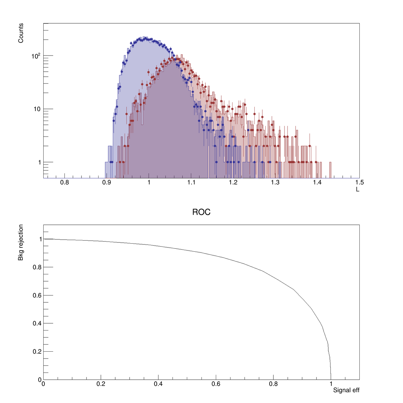
- For each event in the Validation sample we then compute the likelihood ratio, and plot its distribution for the two classes.
- We can then compute the confusion matrix and the ROC (by varying the threshold \(k\) and measuring the true-positive rate vs the false-negative rate for each \(k\) value)
The split between two samples allows us to check for overfitting (i.e. if the classifier distributions don't agree between the two samples, we might have problems)
Remember: after you compute the p.d.f. they should have unitary integral!
Lesson 04
Boosted Decision Trees
Why?
Likelihood classifiers are often not powerful enough.
In addition, they fall short for several reasons:
- Curse of high dimensionality: The more variables you have the more data you need to train one. Especially if you don't settle for 1D projections but you want to build a proper multivariate likelihood.
- Correlation between variables is hard to account for (basically for the same reason)
- They are suboptimal when the separation between signal and background is weak.
Several techniques can perform much better:
Suppor vector machines, Boosted decision trees, Dense neural networks, etc...
Decision trees
Let's start with a classical cut-based analysis
You might start by choosing a variable, applying a threshold and keeping only events above/below the threshold.
Rinse and repeat with another variable, until you reach the desired purity.
The only problem is that with each variable \(i\) you cut on, you select events with some efficiency \(\varepsilon_i\), and the total efficiency after all your selections will be
$$ \varepsilon = \prod_i \varepsilon_i $$
which will decrease significantly unless all your cuts have a very high efficiency...
What if instead of rejecting events if they fail one cut, we continue analyzing them?
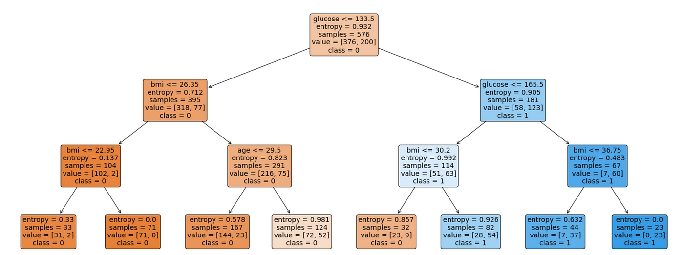
Building a decision tree
Start with the "root" node, it will contain all our events. Then
- Check if some "stopping condition" applies
- For each variable, create a list of all the events in the node, sorted along that variable
- For each list find the optimal splitting point that maximizes sig/bkg separation. If no split improves the separation declare node as "leaf" and break.
- Select variable with the maximal splitting and create two child nodes (one with events that pass, one with events that fail)
- Iterate this procedure on each node
Building a decision tree
This algorithm is "greedy", building on locally optimal choices regardless of the overall result.
At each node all variables are always considered. Even if already used for splitting another node.
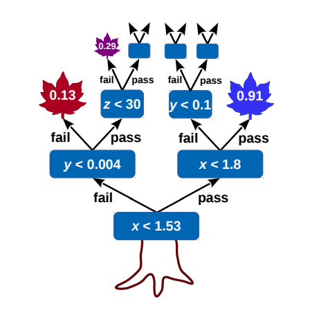
DTs are "human readable". Just a bunch of selections.
To evaluate the tree, follow the cuts depending on each variable value until you reach a leaf node. The result could either be the leaf purity, or a binary decision based on some purity (\(s/s+b\)) threshold.
Decision tree parameters
There are several parameters involved in building a decision tree
- Signal/background normalization, this is basically the relative amount (or weighted relative amount) of signal events and background events. A sample with a 50/50 population is said to be "balanced".
However, this affects only the top nodes of the tree since deeper nodes tend to be more balanced anyway (after all the easy cuts are discovered, the more "difficult" ones remain) - Minimum leaf size
To reduce the impact of statistical fluctuations you might choose to avoid splitting a node if the number of events is below a given threshold - Maximum tree depth
To reduce tree complexity and mitigate overfitting
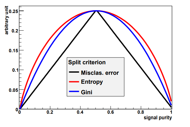
Our choice for splitting points should be based on some solid principles. For example, we might choose to split depending on the value of some function, related to the node impurity. Such a function should be:
- Maximal if the node is balanced (50% signal, 50% background)
- Minimal if the node only contains events from a single class
- Symmetrical w.r.t. signal and background
- Strictly concave (should favor purer nodes)
Then we can quantify how much the separation improves after a split by evaluating the "impurity decrease" for a split \(S\) on a node \(t\)
$$ \Delta i(S,t) = i(t) - p_P i(t_P) - p_F i(t_F)$$
where \(p_{P/F}\) is the fraction of events that pass/fail the split condition. Our goal then reduces to finding the optimal split \(S^*\) such that
$$ \Delta i(S^*,t) = \max_{S \in \{\text{splits}\}} i(S, t) $$
Some common choices for the impurity function:
- Misclassification error \(i(t) = 1 - \max(p, 1-p)\)
- Cross entropy \(i(t) = \sum_{i=s,b}p_i \log(p+i)\)
- Gini index
Variables
Decision trees are particularly good at dealing with high number of variables, and are resilient to many problems that affect other classifiers
- They are less sensitive to the "curse of dimensionality". Training time \(\propto nN \log N\) where \(n\) is the number of variables and \(N\) the number of events.
- They are invariant under monotone transformation of any variable
- They are immune to the presence of duplicate variables
- They can handle both continuous and discrete variables
- They can handle correlation between variables, even if suboptimally
That being said, they have a shortcomings as well, for example:
- They are very sensitive to the training sample composition (adding just a few events might result in completely different splits)
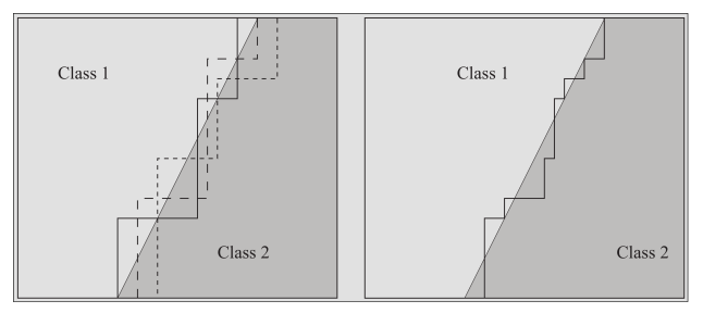
Ensemble learning
Trees can overfit, as any classifier, and there are several methods to mitigate this
- Early stopping
Already discussed, though stopping early might prevent further improvement - Pruning
Remove overly specialized branches to mitigate overfitting, does not help with training stability - Ensemble learning
Helps with stability: train several weak classifiers and leverage their collective results to build a more powerful classifier.
Several kind of ensemble learning for DTs:
- Bagging (bootstrap several subsamples for tree training)
- Random forests (create random training subsamples)
- Boosting
Boosting
Boosting attempts building trees that are progressively more specialized in classifying previously misclassified events.
Let's take a look at the first implementation as an example:
- Train tree \(T_1\) on a sample with \(N\) events
- Train tree \(T_2\) on a new sample with \(N\) events where half were misclassified by \(T_1\)
- Train tree \(T_3\) on a sample with events where \(T_1\) and \(T_2\) disagree
- Take the majority vote between \(T_1\), \(T_2\), \(T_3\) as the resulting classifier
This initial idea can be further generalized
Boosting
Consider a number \(N_\text{tree}\) of classifiers, where the \(k\)-th tree has been trained on sample \(\mathcal T_k\) with \(N_k\) events. Each event has a weight \(w^k_i\) and variables \(\mathbf x_i\), with class \(y_i\).
Now, for each sample \(k\)
- Train classifier \(T_k\) on sample \(\mathcal T_k\)
- Compute weight \(\alpha_k\)for classifier \(T_k\)
- "Transform" sample \(T_k\) in sample \(T_{k+1}\)
The final classifier output will be a function \(F(T_1, ..., T_{N_\text{tree}})\), tipically a weighted average
$$ \lambda_i = \sum_{k=1}^{N_\text{tree}} \alpha_k T_k (\mathbf x_i) $$
and will be an almost-continuous variable
AdaBoost
Take tree \(T_k\) and let us write the misclassification for event \(i\) as
$$ m_i^k = \mathcal I (y_i T_k(\mathbf x_i) < 0) $$
or (in case the tree output is the purity)
$$m_i^k = \mathcal I (y_i [T_k(\mathbf x_i)-0.5] < 0) $$
where \(\mathcal I(X)\) is 1 if \(X\) is true and 0 otherwise.
This way we can define the misclassification rate as
$$ R(T_k) = \varepsilon_k = \frac{\sum_{i=1}^{N_k} w_i^k m_i^k}{\sum_{i=1}^{N_k} w_i^k} $$
and assign the weight to the tree
$$ \alpha_k = \beta \log \frac{1 - \varepsilon_k}{\varepsilon_k} $$
where \(\beta\) is a free parameter (often called learning rate)
AdaBoost
Now we can create the sample for the next tree by just adjusting the weight of each event
$$ w_i^k \rightarrow w_i^{k+1} = w_i^k e^{\alpha_k m_i^k} $$
Note how the weight increases only for misclassified events! Trees become increasingly focused on wrongly labelled events and will try harder to correctly classify them
The final output will then be
$$ \lambda_i = \frac{1}{\sum_k \alpha_k} \sum_k \alpha_k T_k (\mathbf x_i) $$
Interesting side note:
$$ \varepsilon \leq \prod_k 2 \sqrt {\varepsilon_k (1 - \varepsilon_k)} $$
which means that it goes to zero with \(N_\text{tree} \rightarrow \infty\) , which means overfitting
Gradient boosting
Another way to approach the same problem is to turn it into a minimization problem, where adding trees will go towards decreasing a chosen loss function
Let's take the classifier at step \(k\), \(T_k\), we aim now to improve it incrementally
$$ T_{k+1} (\mathbf x) = T_k(\mathbf x) + h(\mathbf x) $$
Now, instead of training a new classifier T_{k+1} we choose to train another classifier, specialized in fitting the residual \(h(\mathbf x)\)
This particular formulation can be seen as minimizing a quadratic loss function of the form
$$ L(\mathbf x, y) = \frac{1}{2} (y - T(\mathbf x))^2 $$
in fact
$$ \frac{\partial L}{\partial T(\mathbf x)} = T(\mathbf x) - y $$
It can be shown that AdaBoost can be recovered as a special case in which
$$ L(\mathbf x, y) = e^{-y T(\mathbf x)}$$
Lecture 04b
We will use the TMVA framework inside ROOT to build our tree(s). It will help us automate a lot of what we've seen so far, so that we don't have to worry with implementing everything from scratch this time.
Lecture 04b
We will use the TMVA framework inside ROOT to build our tree(s). It will help us automate a lot of what we've seen so far, so that we don't have to worry with implementing everything from scratch this time.
Let's see how we can train a BDT. We start with loading the TMVA library and creating a factory object.
TMVA::Tools::Instance();

auto factory = std::make_unique<TMVA::Factory>(
    "StatExam", output_tfile,
    "!V:!Silent:Color:DrawProgressBar:Transformations=I;D;P;G,D:AnalysisType=Classification");
Lecture 04b
We will use the TMVA framework inside ROOT to build our tree(s). It will help us automate a lot of what we've seen so far, so that we don't have to worry with implementing everything from scratch this time.
Let's see how we can train a BDT. We start with loading the TMVA library and creating a factory object. Then we create a "dataloader".
TMVA::Tools::Instance();

auto factory = std::make_unique<TMVA::Factory>(
    "StatExam", output_tfile,
    "!V:!Silent:Color:DrawProgressBar:Transformations=I;D;P;G,D:AnalysisType=Classification");

auto dataloader = std::make_unique<TMVA::DataLoader>("dataset");
Lecture 04b
We then need to inform the dataloader about the variables in our dataset
// for each variable:
dataloader->AddVariable(variable_name, variable_title, "", 'F');
Lecture 04b
We then need to inform the dataloader about the variables in our dataset
// for each variable:
dataloader->AddVariable(variable_name, variable_title, "", 'F');
You can even define new variables as combination of existing ones
dataloader->AddVariable("var1 + (var2 / 3)", "Combined variable", "", 'F');Lecture 04b
We then need to inform the dataloader about the variables in our dataset
// for each variable:
dataloader->AddVariable(variable_name, variable_title, "", 'F');
You can even define new variables as combination of existing ones
dataloader->AddVariable("var1 + (var2 / 3)", "Combined variable", "", 'F');then, add the two trees to the dataloader and let it "prepare" the training and validation sets
dataloader->AddSignalTree(tree_sig);
dataloader->AddBackgroundTree(tree_bkg);

dataloader->PrepareTrainingAndTestTree("", "SplitMode=Alternate:NormMode=NumEvents:!V");
Lecture 04b
We then need to inform the dataloader about the variables in our dataset
// for each variable:
dataloader->AddVariable(variable_name, variable_title, "", 'F');
You can even define new variables as combination of existing ones
dataloader->AddVariable("var1 + (var2 / 3)", "Combined variable", "", 'F');then, add the two trees to the dataloader and let it "prepare" the training and validation sets
dataloader->AddSignalTree(tree_sig);
dataloader->AddBackgroundTree(tree_bkg);

dataloader->PrepareTrainingAndTestTree("", "SplitMode=Alternate:NormMode=NumEvents:!V");
the parameters you see manage how the two sets are created:
- You can apply a "selection cut" (empty in the example)
- We are choosing to alternately assign each event to training or validation, in order, and to split the sets in half, keeping the original signal/background balance.
Check Section 3.1.4 of the TMVA manual for all the possible options
Lecture 04b
Now let's add a classification method from our factory
factory->BookMethod(dataloader.get(), TMVA::Types::kBDT, "BDT_R",
                    "!H:!V:NTrees=250:MinNodeSize=1.0%:MaxDepth=3:BoostType=AdaBoost:AdaBoostBeta=0.5:"
                    "SeparationType=GiniIndex:nCuts=50");
here you have a lot of parameters to choose and possibly optimize, some of will you should recognize already.
Check section 8.13 of the TMVA manual for a detailed explanation.
You can repeat this step, each time adding a new classifier that will be trained. Just remember to give it a different name (third parameter).
Final step: start the training and let TMVA compute the performance of all booked classifiers
// Train MVAs using the set of training events
factory->TrainAllMethods();

// Evaluate all MVAs using the set of test events
factory->TestAllMethods();

// Evaluate and compare performance of all configured MVAs
factory->EvaluateAllMethods();
Lecture 04b
At the end, the factory will write all the results in the TFile you provided as third argument in the factory constructor.
Inside you will find several directories with useful info.
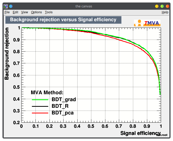
There will be one "Method_" directory for each classifier you trained, and from there you can access the ROC and other properties of the classifier.
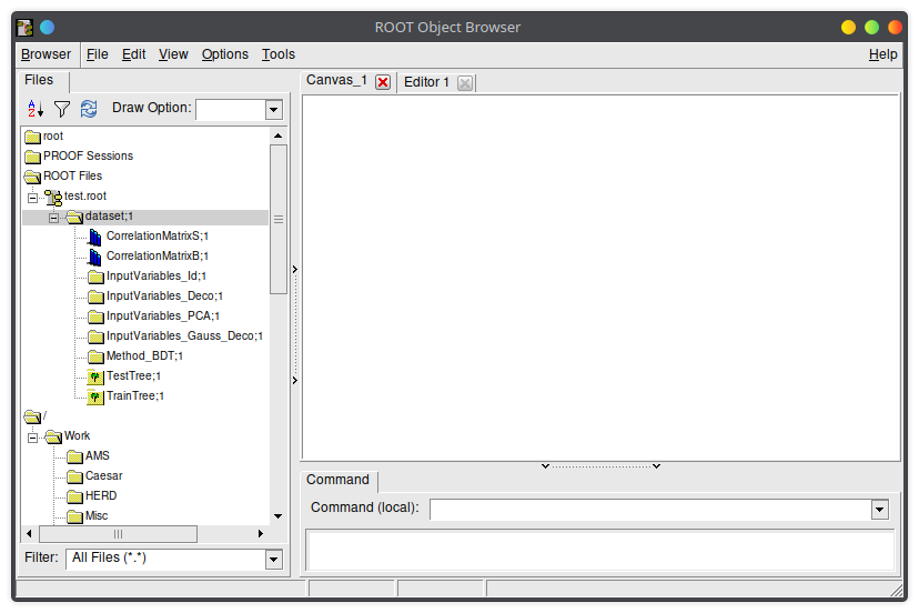
Lecture 04b
You can run the TMVA GUI to inspect the result of the training
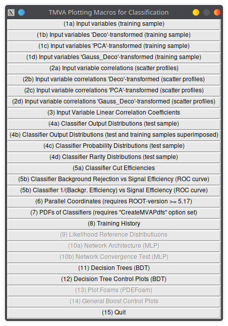
// run in the root interpreter
TMVA::TMVAGui("output_file.root")
Lecture 04b
You can run the TMVA GUI to inspect the result of the training.
For example:
- visualize the training set
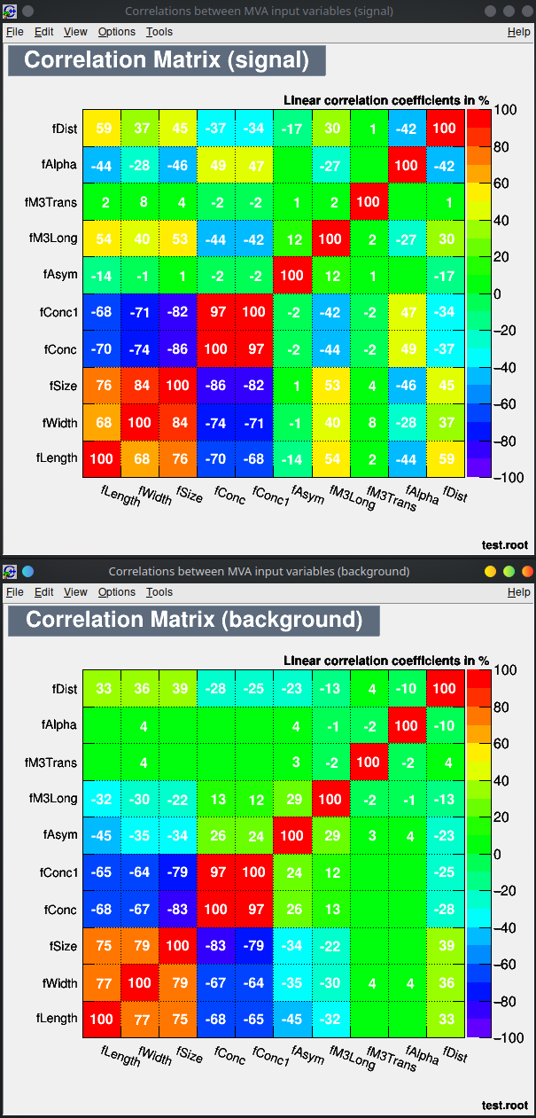
- visualize correlations in the training set
- check the results of your training
Lecture 04b
You can run the TMVA GUI to inspect the result of the training.
For example:
- visualize the training set
- visualize correlations in the training set
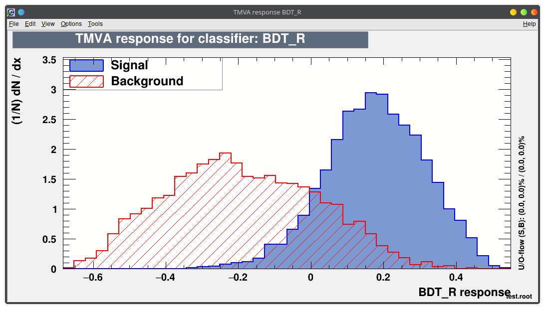
- check the results of your training
- visualize each BDT
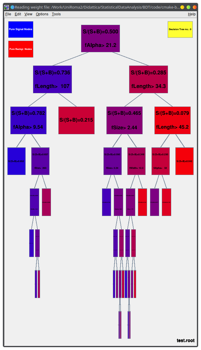
Lecture 04b
Train your BDTs!
Choose different parameters, try AdaBoost vs Gradient Boosting, or a different impurity function for splitting.
Document what you see and compare the results in your report.
Main goal: compare the ROC curves you get with the one from your homemade likelihood, and try to explain how and why they differ.
2023 - Classification exercise
By Valerio Formato


