Multilevel Modeling, Part 2
PSY 356
Multilevel models for longitudinal data
- Nationally representative survey of \(N=6504\) adolescents
- Each followed up for a maximum of five time points
- Ages at the first time point ranged from 13 to 21.
- Ages at the fifth time point ranged from 35 to 42.
- We are using data from the first four time points.
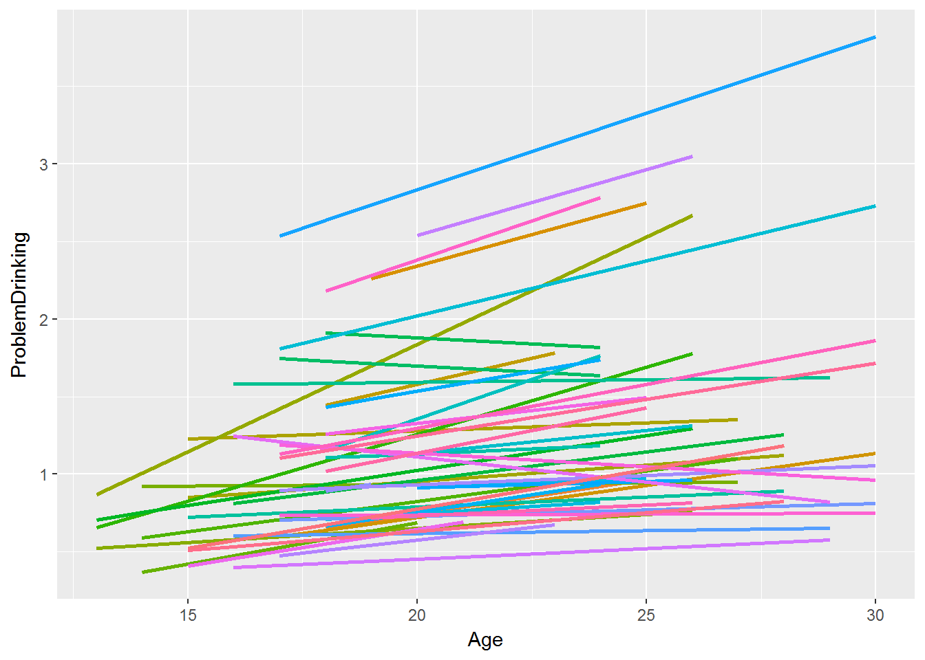
- Here, we predict drinking score, a composite score of three drinking-related indicators, from adolescence through early adulthood.
Motivating Example: Add Health
Drinking_{ij} = \beta_{0j} + \beta_{1j}Age_{ij} + r_{ij}
\beta_{0j} = \gamma_{00} + u_{0j}
\beta_{1j} = \gamma_{10}
u_{0j}\sim N\left(0,\tau_{00}\right)
r_{ij}\sim N\left(0,\sigma^2\right)
Level 2
Level 1
Random-intercept model
Here, \(Age_{ij}\) and \(Drinking_{ij}\) are the age and drinking score, respectively, of subject \(j\) at time \(i\), and Note that under this formulation, only the intercept can vary by person.
Drinking_{ij} = \beta_{0j} + \beta_{1j}Age_{ij} + r_{ij}
\beta_{0j} = \gamma_{00} + u_{0j}
\beta_{1j} = \gamma_{10} + u_{1j}
\begin{bmatrix}
u_{0j} \\
u_{1j}
\end{bmatrix}
\sim N
\begin{bmatrix}
\tau_{00} & \\
\tau_{01} & \tau_{11}
\end{bmatrix}
r_{ij}\sim N\left(0,\sigma^2\right)
Level 2
Level 1
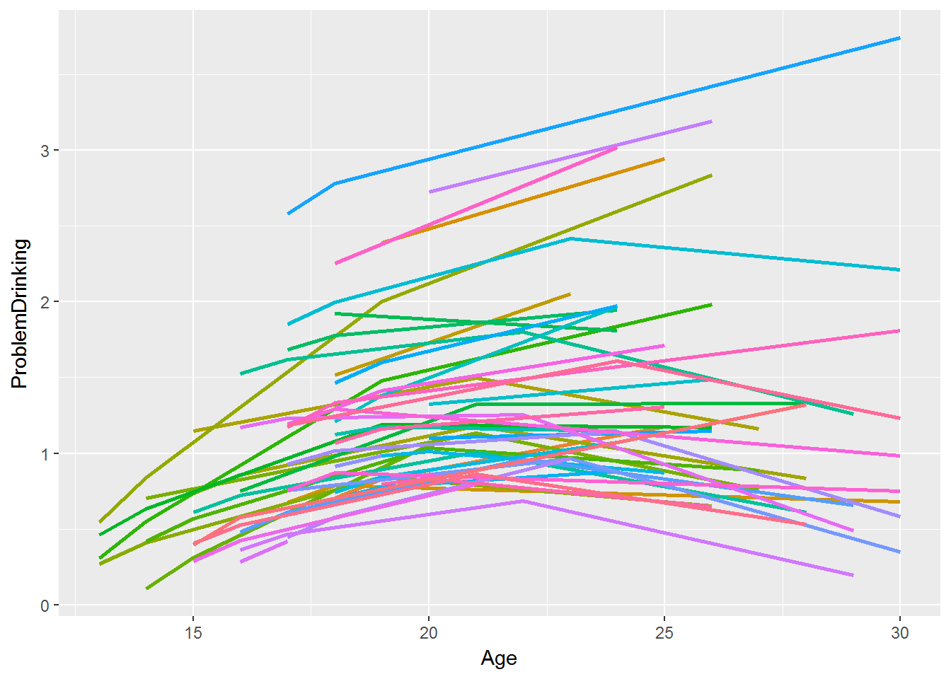
Random-slopes model
Now, under this formulation, we can have variation in the slopes by person.
- For linear growth, we can just put age in there, or we can alter it any number of ways:
- We can subtract out the first time
- We can rescale it by some multiple (e.g., 10)
- Sometimes this helps with convergence
- We can also enter a quadratic component of time - i.e., \(age^2\).
- Or cubic (\(age^3\)), quartic (\(age^4\)), not sure if quintic (\(age^5\)) is a word but let's go with it...
- Note that if you enter in a polynomial, you must include all lower-order polynomials.
How does time enter the model?
Drinking_{ij} = \beta_{0j} + \beta_{1j}Age_{ij} + \beta_{2j}Age^2_{ij} + r_{ij}
\beta_{0j} = \gamma_{00} + u_{0j}
\beta_{1j} = \gamma_{10} + u_{1j}
\begin{bmatrix}
u_{0j} \\
u_{1j}
\end{bmatrix}
\sim N
\begin{bmatrix}
\tau_{00} & \\
\tau_{01} & \tau_{11}
\end{bmatrix}
r_{ij}\sim N\left(0,\sigma^2\right)
Level 2
Level 1
Adding a quadratic component
This can help us to model change that increases and subsequently decreases or levels off. Note that we could include a random effect for that quadratic component too.
\beta_{2j} = \gamma_{20}
-
Level 2: We can add person-level predictors by allowing the intercept, slope, or both to vary for different people.
- Again, this is the same as the intercepts-as-outcomes and slopes-as-outcomes model, but don't worry too much about the terminology.
-
Level 1: We can add a time-level predictor, but note that the interpretation of these coefficients can be challenging.
- If a variable is contemporaneous with the outcome, it can be challenging to make causal statements.
Predictors
Drinking_{ij} = \beta_{0j} + \beta_{1j}Age_{ij} + r_{ij}
\beta_{0j} = \gamma_{00} + \gamma_{01}Male_j + u_{0j}
\beta_{1j} = \gamma_{10} + u_{1j}
\begin{bmatrix}
u_{0j} \\
u_{1j}
\end{bmatrix}
\sim N
\begin{bmatrix}
\tau_{00} & \\
\tau_{01} & \tau_{11}
\end{bmatrix}
r_{ij}\sim N\left(0,\sigma^2\right)
Level 2
Level 1
Adding predictors
Now we have the intercept of drinking being allowed to differ between males and females. We could also allow the slopes to differ.
Special cases
The paired samples t-test examines the difference between paired observations:
$$t = \frac{\bar{d}}{\frac{s_d}{\sqrt{n}}}$$
Where:
- \(d_i = y_{i1} - y_{i0}\) (difference between paired observations)
- \(\bar{d}\) is the mean of differences
- \(s_d\) is the standard deviation of differences
- \(n\) is the number of pairs
Paired-samples t-tests as MLM's
We can reframe this as a multilevel model, with measurements nested within subjects:
Level 1
where:
- \(y_{ij}\) is the outcome for subject \(j\) at measurement \(i\)
- \(G_{ij}\) is the dummy-coded group variable (0 = condition 0, 1 = condition 1)
- \(r_{ij}\) is the measurement-level residual
- \(\gamma_{00}\) is the average outcome in condition 0
- \(\gamma_{10}\) is the average difference between conditions
- \(u_{0j}\) are subject-level random effects
$$\beta_{0j} = \gamma_{00} + u_{0j}$$
$$y_{ij} = \beta_{0j} + \beta_{1j}G_{ij} + r_{ij}$$
Level 2
$$\beta_{1j} = \gamma_{10}$$
- \(\gamma_{10}\) is equivalent to \(\bar{d}\) in the paired t-test
- Testing \(H_0: \gamma_{10} = 0\) is equivalent to the paired t-test
- Critical note: standard paired-samples t-test does NOT include random slope
- The multilevel approach allows for:
- Missing data
- Inclusion of covariates
- More complex variance structures
Interpretation
Repeated measures ANOVA examines differences across multiple conditions within subjects:
$$ F = \frac{MS_{group}}{MS_{error}} = \frac{\frac{SS_{group}}{df_{group}}}{\frac{SS_{error}}{df_{error}}} $$
where:
- \( SS_{group} \) is the sum of squares for group effect
- \( SS_{error} \) is the sum of squares for error
- \( df_{group} = k - 1 \) (\( k \) is the number of conditions)
- \( df_{error} = (N-1)(k-1) \) (N is the number of subjects)
Key assumption: Sphericity (equal variances of differences between all pairs of conditions)
Repeated-measures ANOVA's as MLM's
We can reframe this as a multilevel model with measurements nested within subjects:
$$y_{ij} = \beta_{0j} + \sum_{m=1}^{k-1} \beta_{mj}G_{mij} + r_{ij}$$
$$\beta_{0j} = \gamma_{00} + u_{0j}$$
$$\beta_{mj} = \gamma_{m0}$$
where:
- \( y_{ij} \) is the outcome for subject \( j \) at measurement occasion \( i \)
- \( G_{mij} \) are dummy codes for conditions (reference is condition 0)
- \( r_{ij} \) is the measurement-level residual with variance \( \sigma^2 \)
- \( \gamma_{00} \) is the average outcome in the reference condition
- \( \gamma_{m0} \) represents mean differences between each condition and reference
- \( u_{0j } \) are subject-level random effects with variance \( \tau^2 \)
Level 1
Level 2
- Testing omnibus hypothesis \( (H_0: \gamma_{10} = \gamma_{20} = ... = \gamma_{(k-1)0} = 0) \) is equivalent to repeated measures ANOVA F-test
- The multilevel approach offers several advantages:
- Handles missing data appropriately
- Allows inclusion of subject-level and time-varying covariates
- Can model more complex variance structures beyond sphericity
- Permits random slopes (allowing treatment effects to vary by subject)
- Accommodates continuous predictors and more complex designs
- Can handle unbalanced designs and irregular measurement occasions
Note: The standard RM-ANOVA assumes compound symmetry and sphericity, while multilevel models can relax these assumptions by specifying different variance-covariance structures.
Interpretation
- Here, we consider a single person as a "group", in the sense that all time points are nested within a given person.
- We will use time as a Level-1 predictor.
- The models we're going over can be considered a special case of structural equation models.
- One piece of advice: don't get too hung up on which piece of MLM jargon (e.g., intercepts-as-outcomes, slopes-as-outcomes) each model maps onto.
Longitudinal data
Thank you!
colev@wfu.edu
Copy of Multilevel Modeling, Part 2
By Veronica Cole


