

Vidhi Lalchand
Postdoctoral Fellow, Broad and MIT
Vidhi Lalchand
11-07-2025
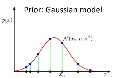
Give data samples \( \{x\}_{n=1}^{N}\), learn the probability distribution of data \(p(x)\).
Once you learn \(p(x)\), you can sample from it to generate new instances of the data, \( x_{new} \sim p(x)\).
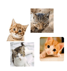
Data can be high-dimensional, like text, speech, images, molecules.
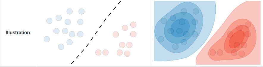
In a discriminative model, we instead directly learn the conditional distribution \(p(y|x)\) i.e. a decision boundary, in the case of classification, or regression models we learn to predict \( y\) from \( x\).
In the presence of labels \(y\), generative models learn the joint probability distribution of data \(p(x, y)\).
Generative models can also perform discriminative tasks.
|
Smith MJ, Geach JE. Astronomia ex machina: a history, primer and outlook on neural networks in astronomy. Royal Society Open Science. 2023 May 31;10(5):221454.
|
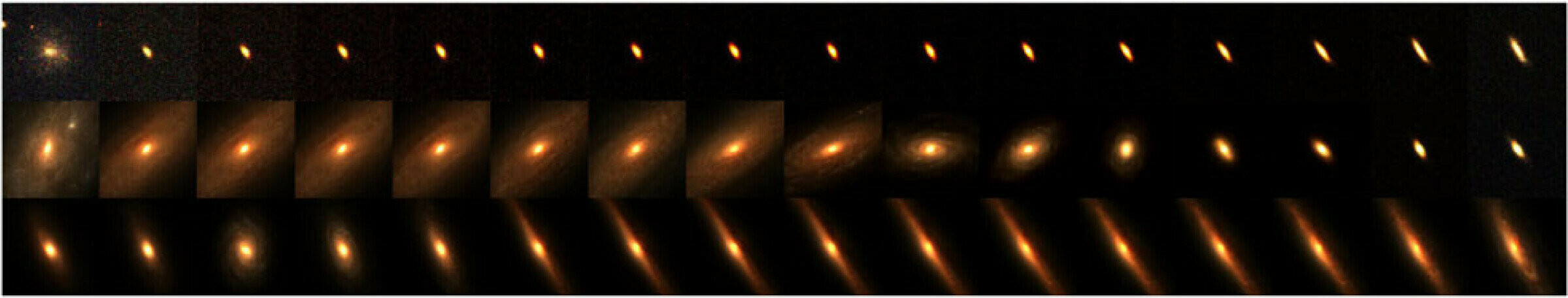
Generative models are powerful tools for embeddings discrete objects into a continuous space, thereby allowing one to simulate them.
Latent space
Interpolating between the continuous representation of astronomical objects in latent space
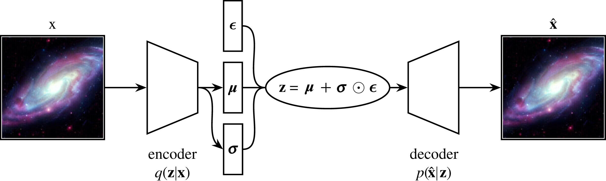
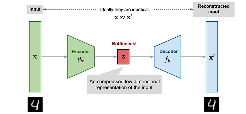
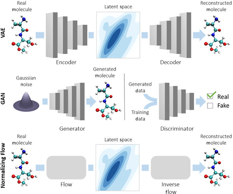
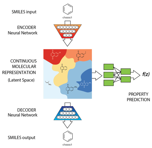
Typical autoencoder style architecture of generative models
Interpolating between the continuous representation of astronomical objects in latent space
Smith MJ, Geach JE. Astronomia ex machina: a history, primer and outlook on neural networks in astronomy. Royal Society Open Science. 2023 May 31;10(5):221454.
Latent variable models (LVMs) are a powerful class of generative models that introduce hidden (latent) variables to explain observed data.
Let \(z\) denote a 2d latent variable [position, radius]
One can generate \( \mathbf{x}\) given \( \mathbf{z}\), \( \mathbf{z} \longrightarrow \mathbf{x}\).
The structure of the data is captured by the compressed latent variable \(\mathbf{z}\), while the data representation in pixels is several hundred dimensions.
\( \mathbf{x}\)
In real data, \( \mathbf{z}\) is not explicitly known, it has to be learnt from the data.
The fundamental assumption underlying LVMs is that the data generation process involves some latent variable \( \mathbf{z}\). The data \(\mathbf{x}\) is generated through \(\mathbf{z}\).
\( \mathbf{x}\)
\( \mathbf{z}\)
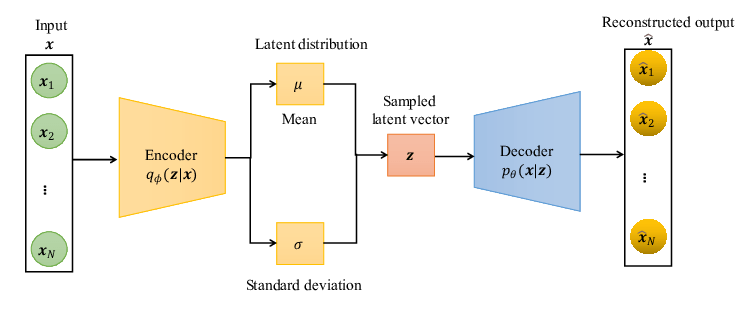
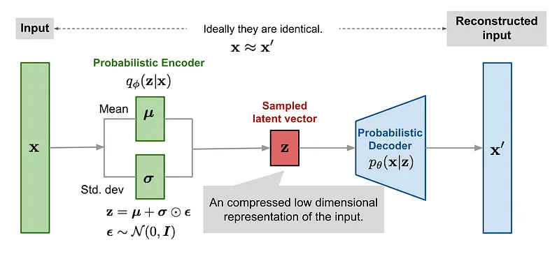
Inference \( q_{\phi}(\mathbf{z}|\mathbf{x})\)
Generation \( p_{\theta}(\mathbf{x}|\mathbf{z})\)
Reconstructed input
In VAEs we want to maximise the ELBO so the loss function is negative of the ELBO.
The reconstruction likelihood encourages the decoder to accurately reconstruct the data from the latent \(\mathbf{z}\).
The KL term forces points to stay close to the prior, exerting a counter weight.
The reconstruction likelihood encourages the decoder to accurately reconstruct the data from the latent \(\mathbf{z}\).
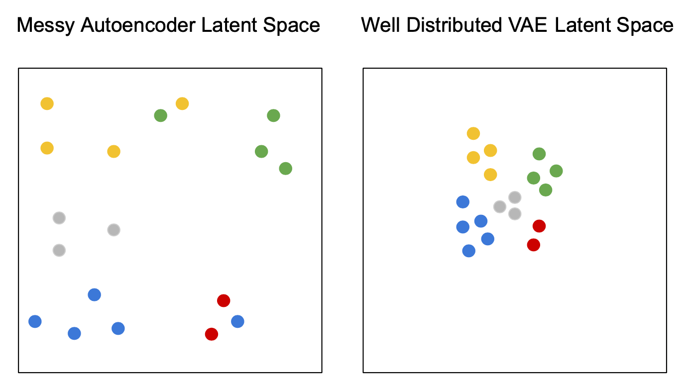
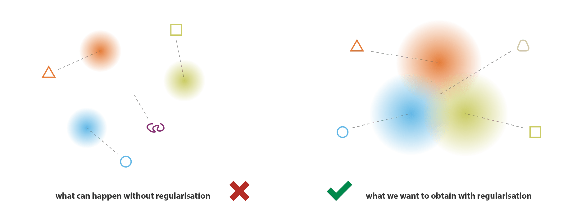
VAEs can be viewed as a "regularised" version of an autoencoder. It is trained to preserve two properties of the latent space:
1. Continuity
2d \(\mathbf{z}\) space
Prior \(p(\mathbf{z}) = \mathcal{N}(0,1)\)
Smooth transitions in latent space should correspond to smooth transitions in data space.
Points in an epsilon-neighbourhood of a reference point should have very similar outputs.
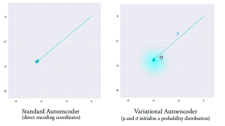
A single encoding of an autoencoder vs. a variational autoencoder in a 2d latent space.
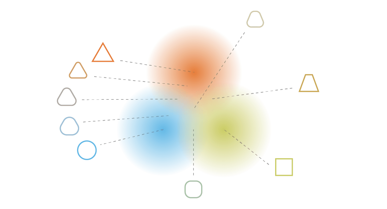
The entire latent space in a VAE comprises these soft ellipsoidal regions denoting Gaussian distributions.
2. Completeness
Sampling randomly from the prior should lead to plausible data instances.
2d \(\mathbf{z}\) space
Autoregressive Generative Models are a paradigm of choice for search and design of new drugs.
It's a widely cited estimate that there are around 106010^{6010
1010010^{100}~\(10^{60}\) chemically valid, synthetically accessible small molecules, even under fairly conservative definitions of "small."
Why is drug-design an interesting problem in the first place?
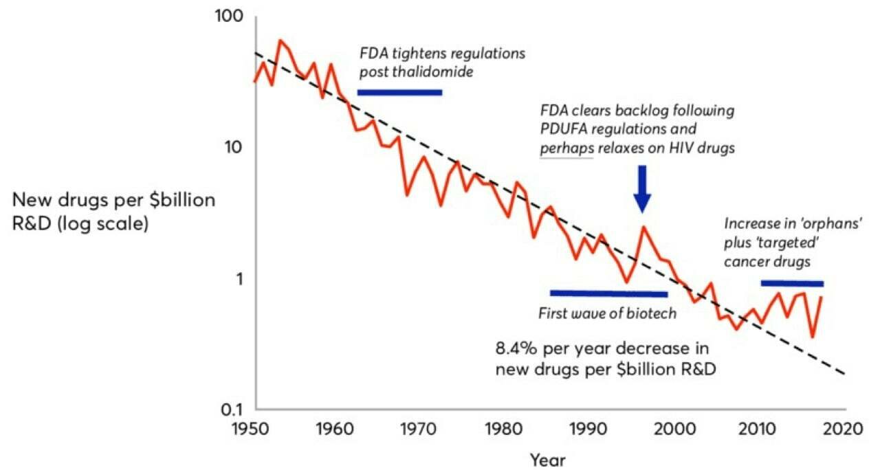
Drug discovery has been witnessing an inverse of Moore's law -- pharma companies are spending increasingly more $ on fewer drugs (drugs brought to market per billion$ of R&D).
Eroom's law!
Roadmap: Unlocking machine learning for drug discovery. Bessember Venture Partners Technical Report, 2021.
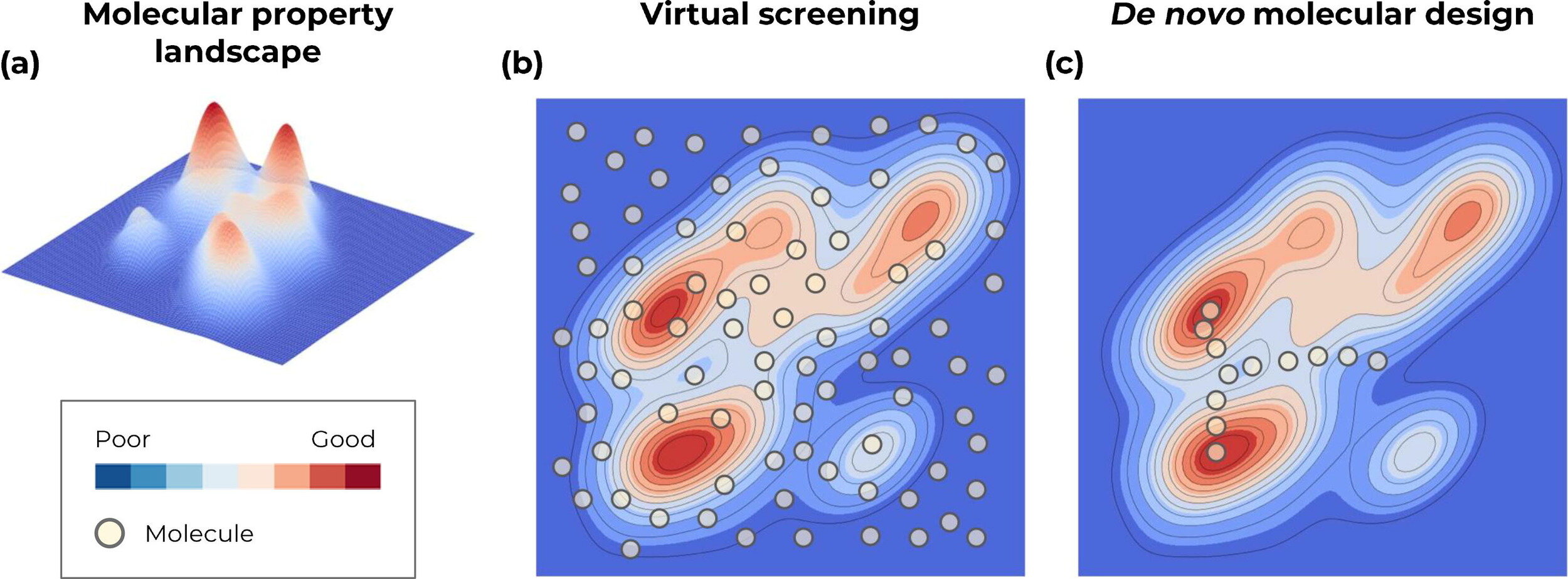
Virtual screening or De novo molecular design
Screen from a finite list of known molecules
Traverse the continuous representation of the chemical space (through optimisation)
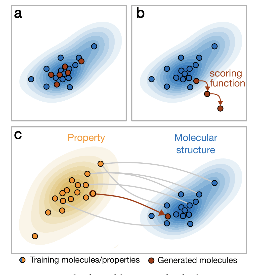
Generative approaches for de novo molecular design
Gómez-Bombarelli R, et al. Automatic chemical design using a data-driven continuous representation of molecules. ACS central science. 2018. (ChemicalVAE)
Kusner MJ et al. Grammar variational autoencoder. InInternational conference on machine learning, 2017. (GrammarVAE)
Jin W et al. Junction tree variational autoencoder for molecular graph generation. InInternational conference on machine learning 2018. (JT-VAE)
De Cao N, Kipf T. MolGAN: An implicit generative model for small molecular graphs. ICML Workshop for Applications of Deep Generative Models. 2018. (MolGAN)
Kang S, Cho K. Conditional molecular design with deep generative models. Journal of chemical information and modeling. 2018. (SSVAE)
Zang C, Wang F. Moflow: an invertible flow model for generating molecular graphs. InProceedings of the 26th ACM SIGKDD international conference on knowledge discovery & data mining 2020. (MoFlow)
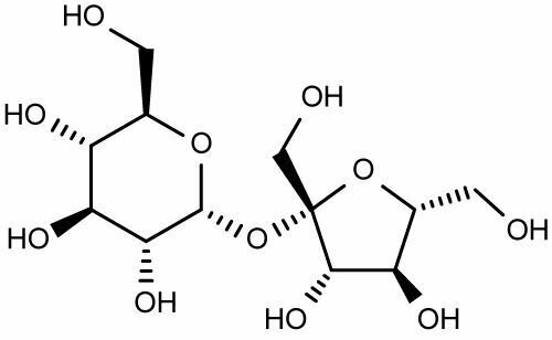
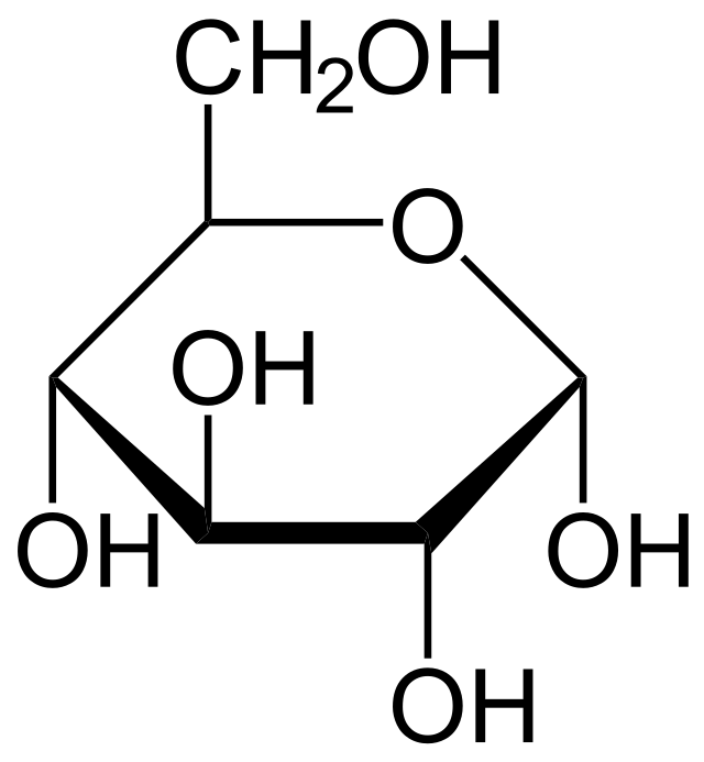
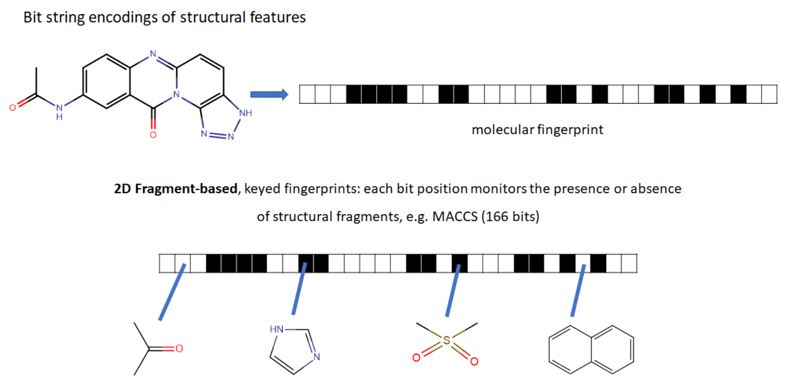
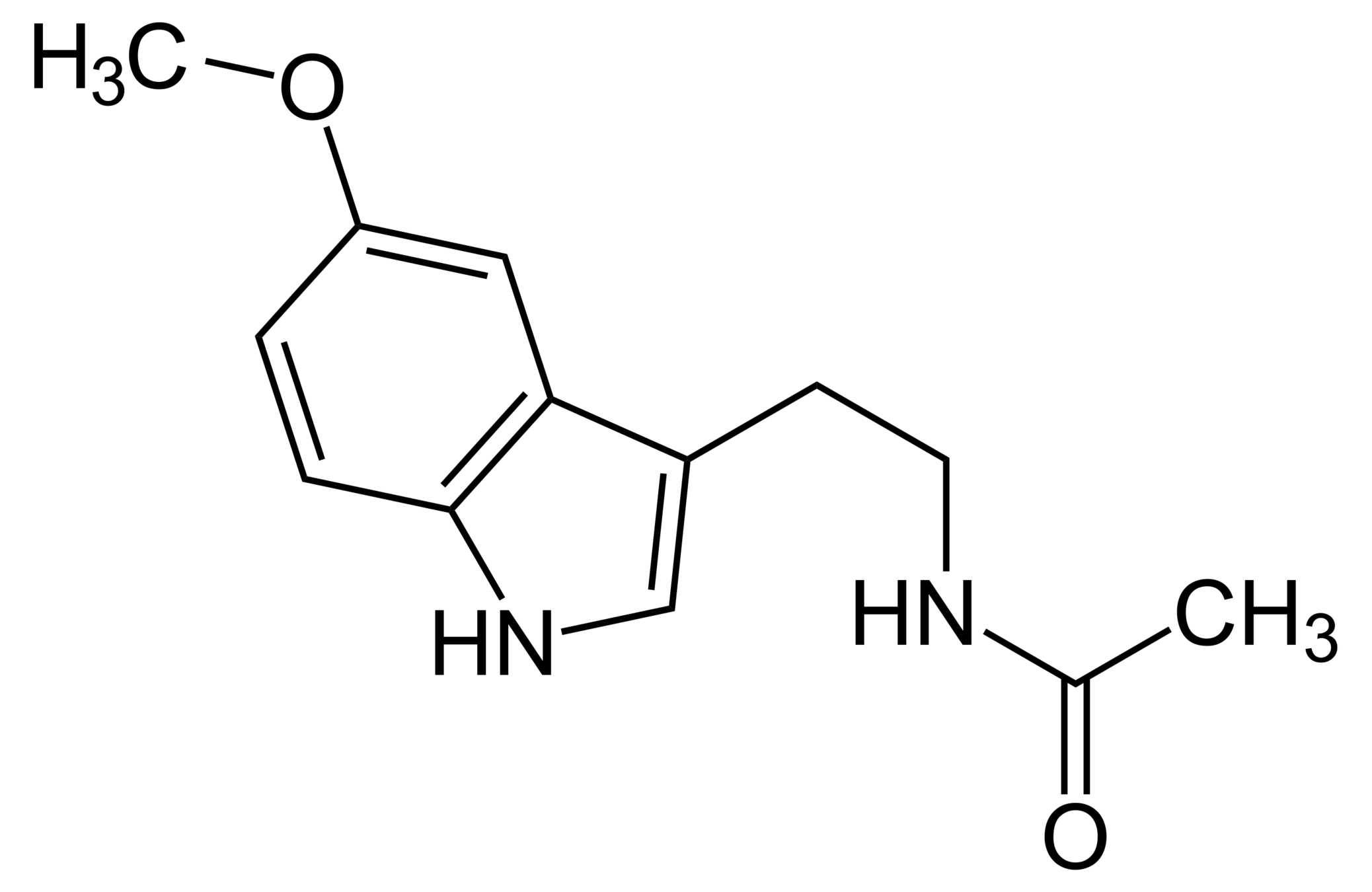
Representation of small drug-like molecules
Understanding how to best represent molecules in a machine-readable format is a key challenge and an active area of research.
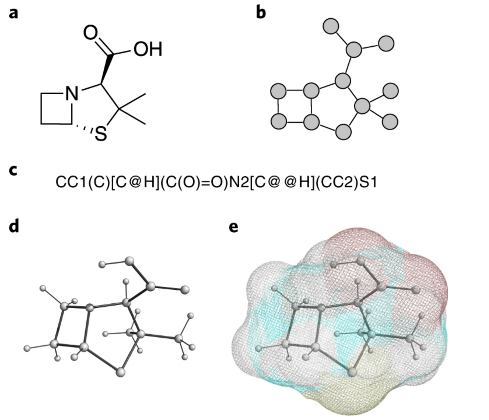
Formally, there are 4 representations which are prevelant in literature:
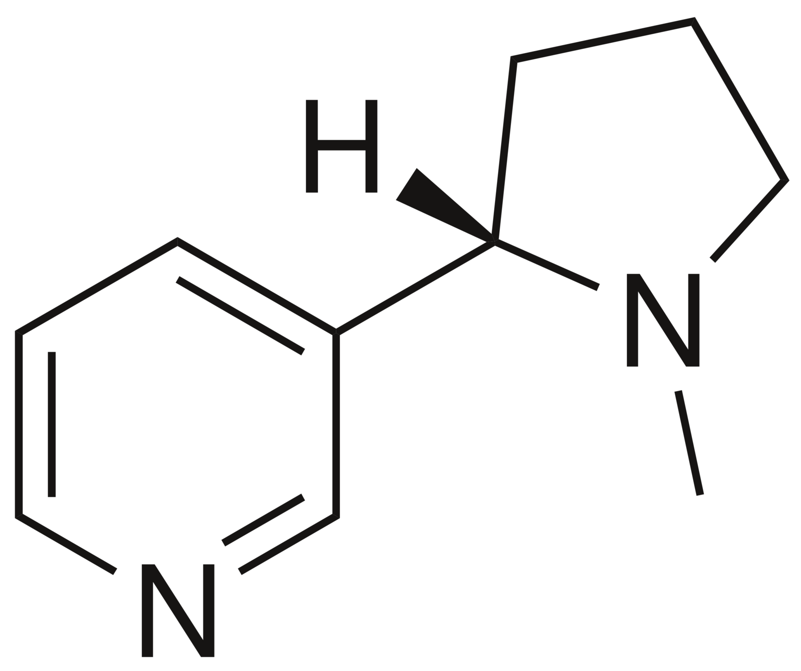
SMILES (Simplified molecular-input line-entry system) is a formalism to generate a string identifier for chemical compounds. It has an alpha-numeric nomenclature which uses atomic letters to denote atoms, parenthesis () to denote branches and symbols =, #,$ to denote double, triple and quadruple bonds.
ECFP (Extended connectivity fingerprints)
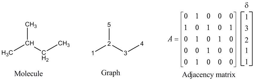
2D graph
3D graph
CC(=O)NCCC1=CNc2c1cc(OC)cc2
CN1CCC[C@H]1c2cccnc2
Melatonin
Nicotine
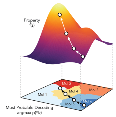
Generative model + Property prediction
How do we use generative modelling to identify molecules which optimise a property of interest?
Gómez-Bombarelli R, et al. Automatic chemical design using a data-driven continuous representation of molecules. ACS central science. 2018. (ChemicalVAE)
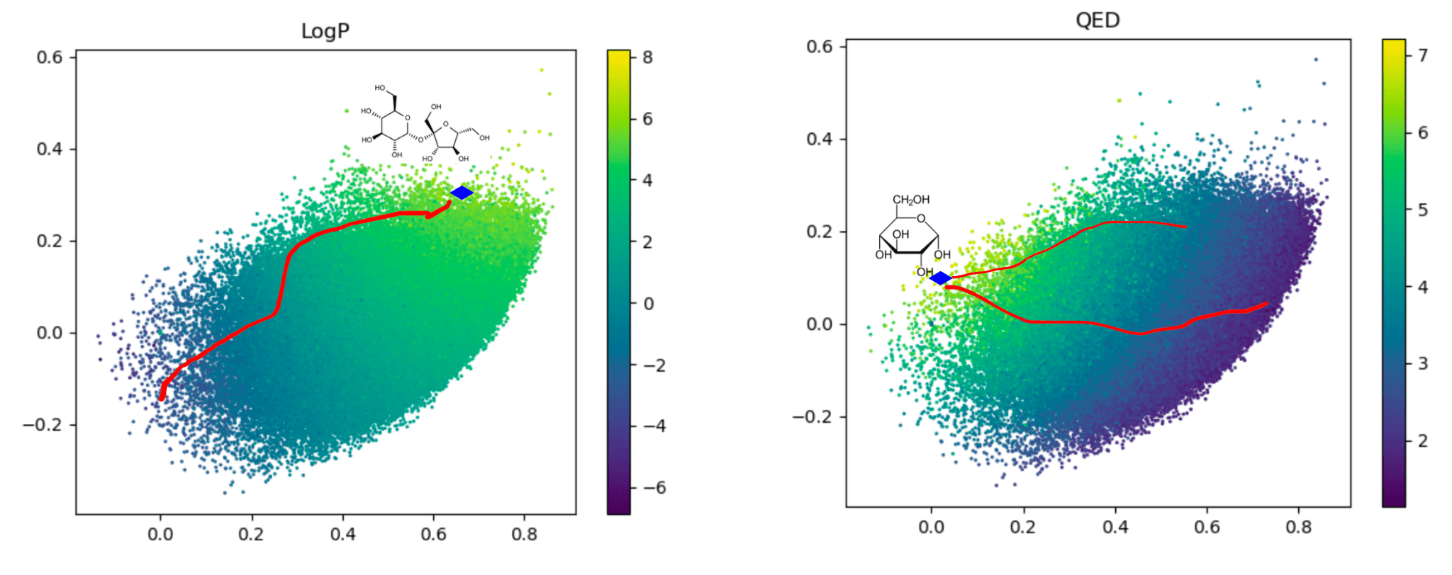
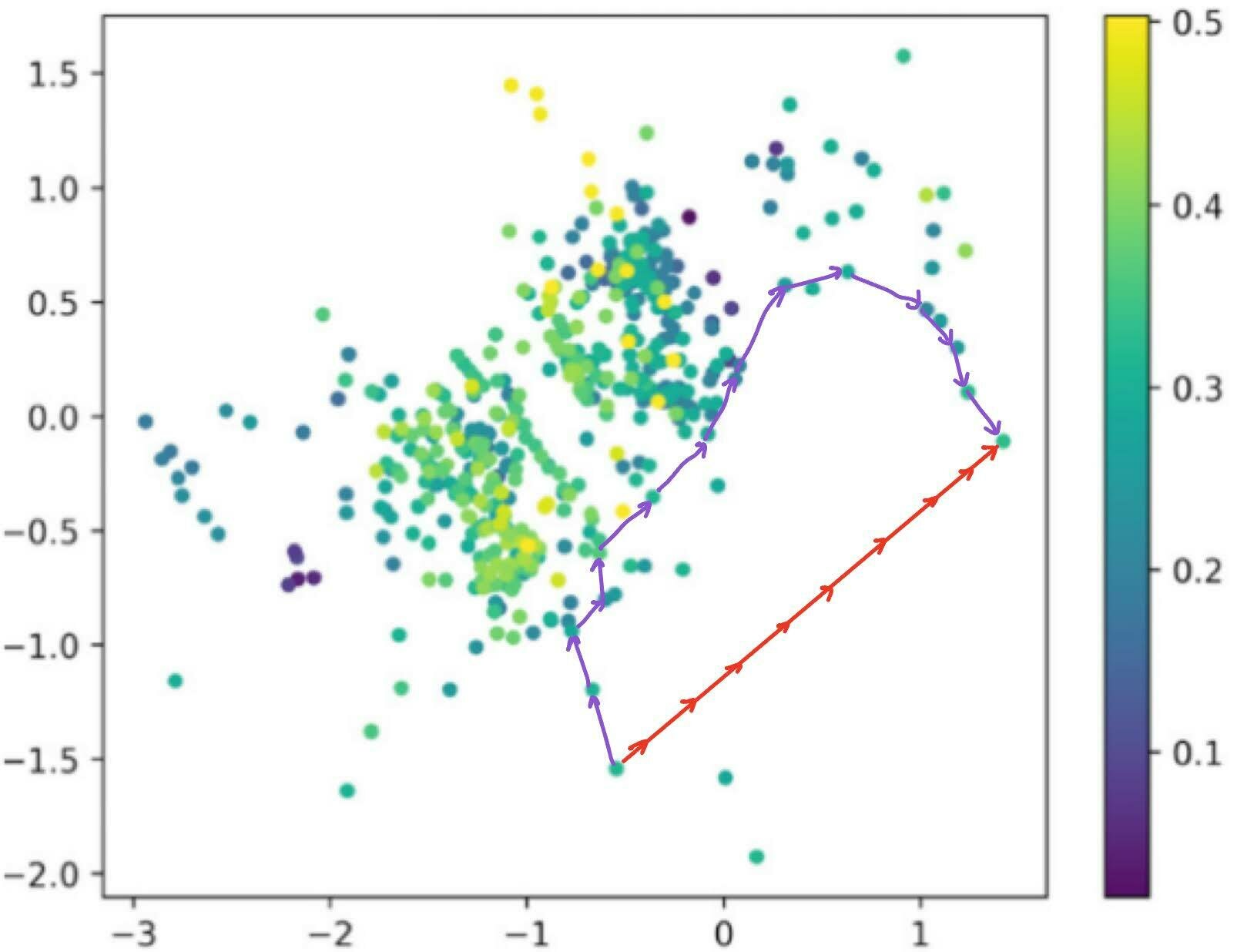
Traversal over a convex subspace of the latent space
Evolution of a 2d subspace of the latent space during training
Points shaded by actual QED (drug-likeness) scores
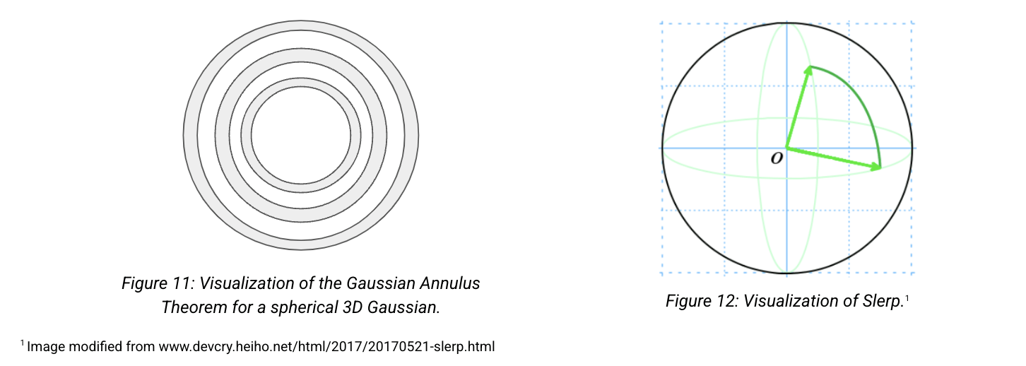
Gaussian Annulus theorem
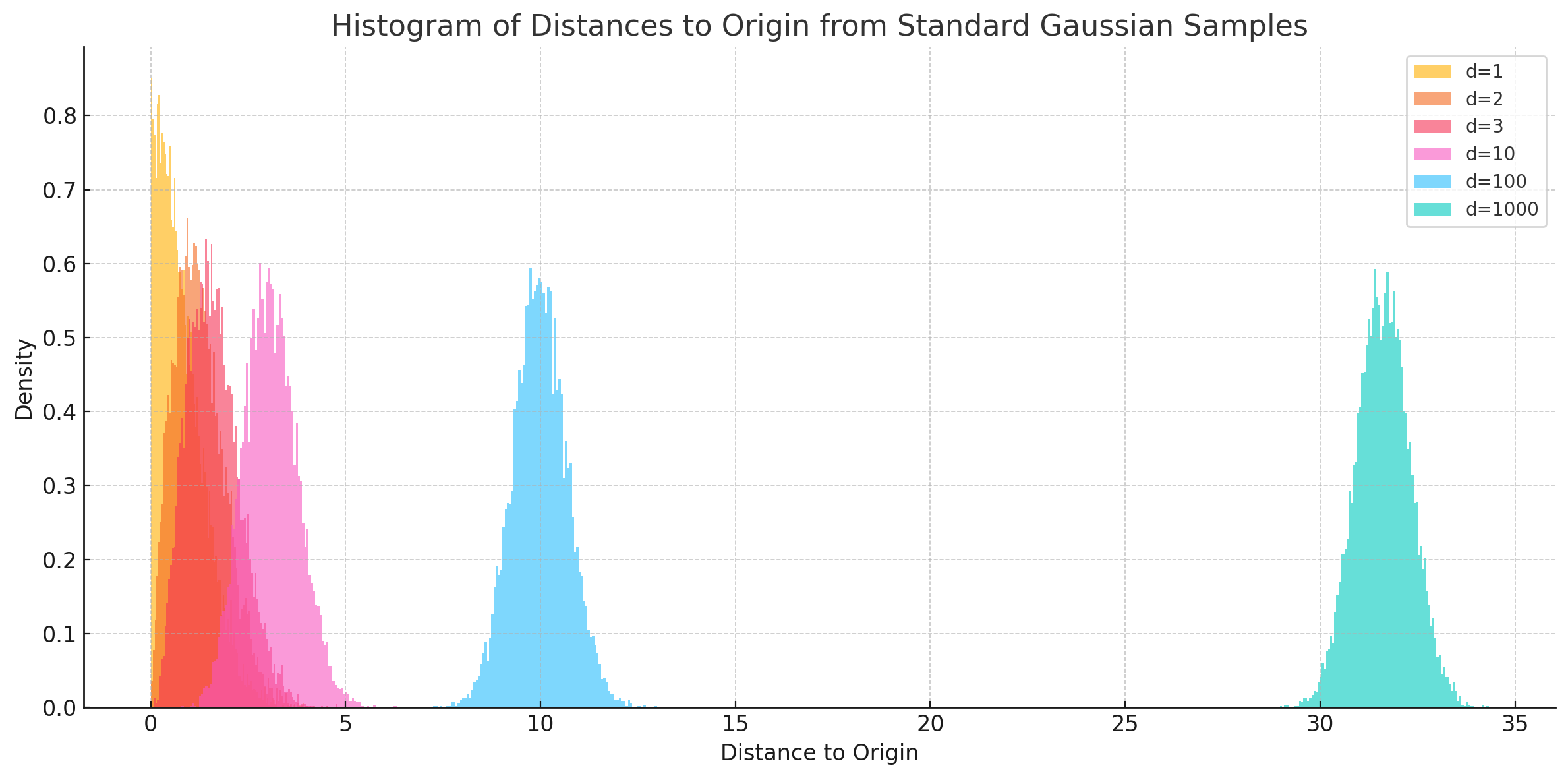
The Gaussian Annulus Theorem tells us that most of the probability mass of a high-dimensional Gaussian lies in a thin shell -- also called, the "soap bubble" effect.
Instead of interpolating between two points by traversing the low-density Euclidean interpolation, traverse across the surface of this high-density shell. This is known as Spherical Linear Interpolation (Slerp).
As, \(d \longrightarrow \infty\), the samples pile up almost equidistant from the origin, giving the shell effect.
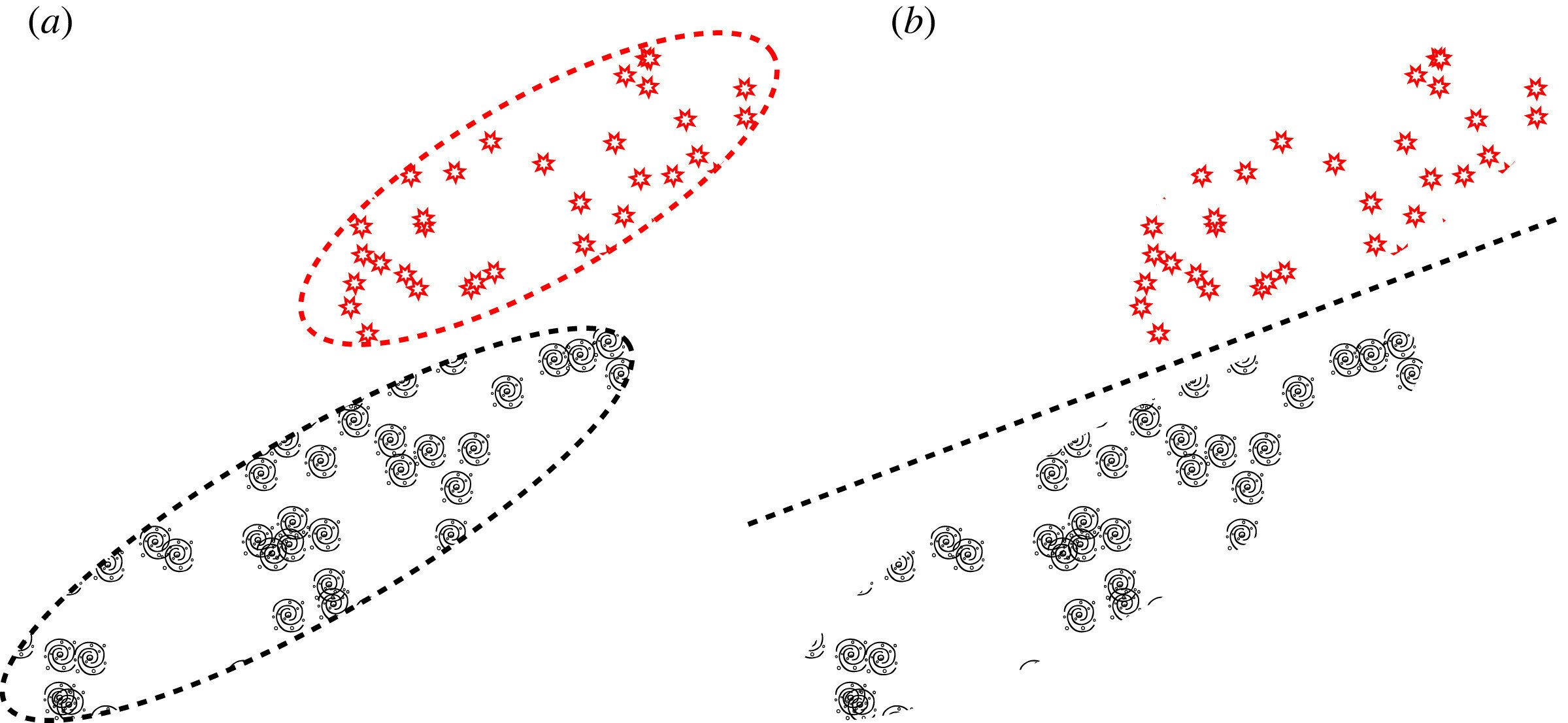
Dead-zones in latent traversals
1 Image modified from ChemNav: An interactive visual tool to navigate in the latent space for chemical molecules discovery (www.doi.org/10.1016/j.visinf.2024.10.002).
2 Image from ChemNav: An interactive visual tool to navigate in the latent space for chemical molecules discovery (www.doi.org/10.1016/j.visinf.2024.10.002).
Dead zones in (a subspace of) the latent space. The Euclidean interpolation (red) visits degenerate latent embeddings, while slerp traces a path through the regions where there is valid data.
| Model | Creator | Train size | Representation | Year |
|---|---|---|---|---|
| Molformer-XL | IBM | 1.1 bn | SMILES | 2022 |
| MegaMolBART | NVIDIA | 1.45 bn | SMILES | 2021 |
| ChemBertA | Reverie Labs | 77 mn | SMILES | 2020 |
| Chemformer | AstraZeneca | 100 mn | SMILES | 2021 |
| MolE | Recursion Pharma | 1.2 mn | Graphs | 2022 |
Pre-training methodology: Self-supervised learning like masked language modelling.
Evaluation: MoleculeNet benchmarks (incl. property prediction) & Therapeutic Data Common benchmarks.
Foundation Models
Open questions: But what about their latent spaces? are they contiguous, smooth, regular? how to traverse them efficiently?
Foundation Models
Key-takeaways
Thank you!
All generative models implicitly learn latent vectors which live on some structured manifold.
embedding spaces (e.g. token/patch embeddings),
latent spaces (in VAEs, diffusion, etc.),
Their representation topology is extremely important, questions like:
Embeddings of large pre-trained models need to be evaluated and studied through the lens of geometry -- curved latent geometry can reflect robustness vs brittleness and different generalisation capabilities.
Do similar inputs lie on connected submanifolds?
Are there geometric clusters for tasks, concepts, or modalities?
What's the intrinsic dimension of representations across layers?
The idea of navigating latent spaces is deeply tied to many frontier problems in biomedical ML.
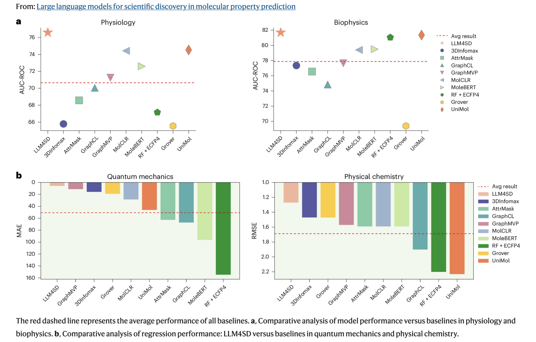
Domain Tasks Metric Gain
| Physiology (e.g., BBBP, Tox21) | 41 | AUC-ROC | ↑2–3% vs. SOTA |
| Biophysics (e.g., HIV, BACE) | 2 | AUC-ROC | ↑2–3% |
| Physical Chemistry (e.g., ESOL, Lipophilicity) | 3 | RMSE | ↓12.9% |
| Quantum Mechanics (QM9) | 12 | MAE | ↓48.2% |
LLM4SD was tested across 58 molecular property prediction tasks from MoleculeNet, spanning four domains.
LLM is prompted:
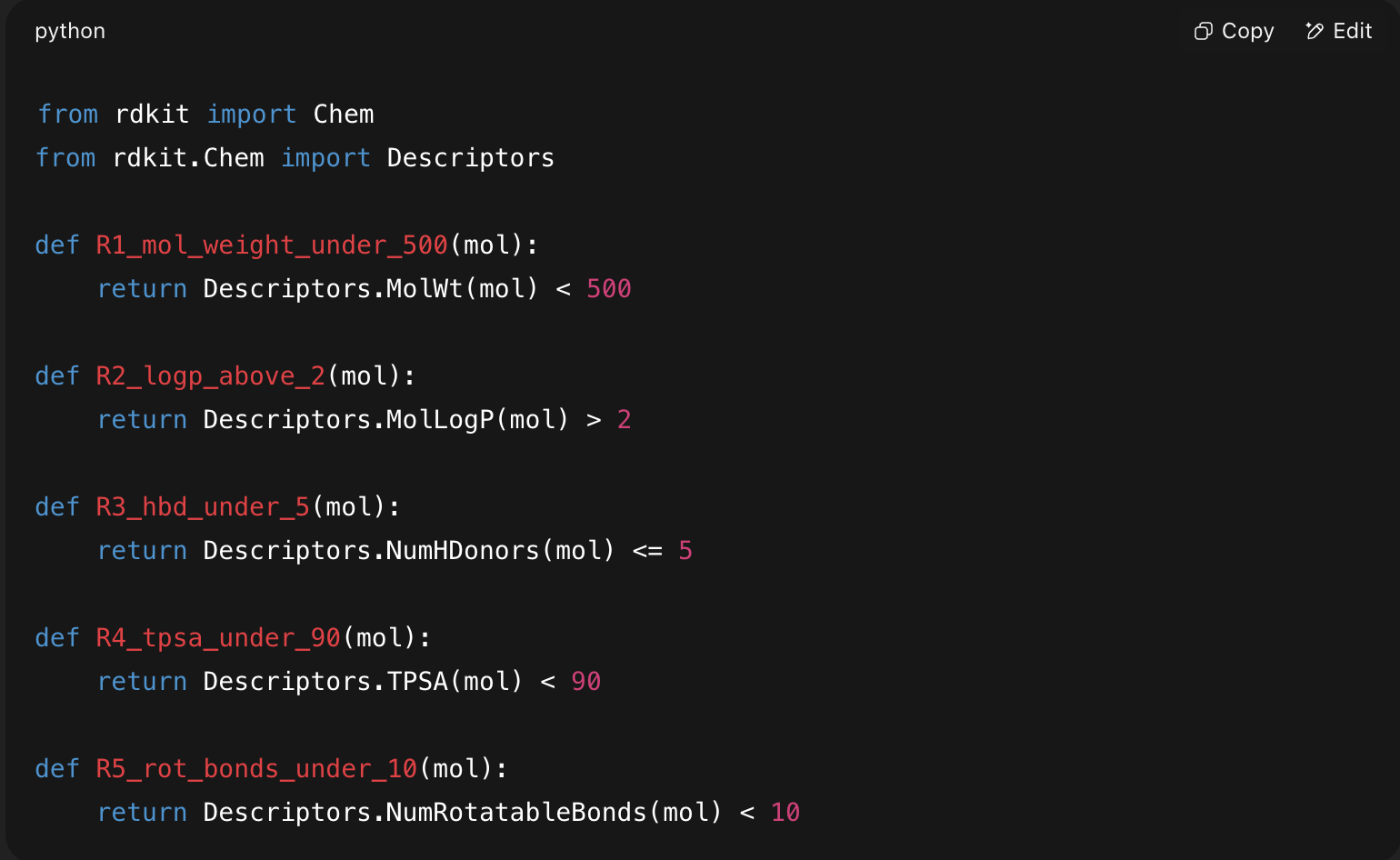
“You are an expert chemist. What rules are useful to predict whether a molecule can cross the blood–brain barrier?”
Rule ID Rule Text
| R1 | Molecular weight < 500 Da |
| R2 | LogP > 2.0 |
| R3 | ≤ 5 hydrogen bond donors |
| R4 | Topological polar surface area (TPSA) < 90 Ų |
| R5 | Fewer than 10 rotatable bonds |
LLM output:
Each rule is written as a Python function using RDKit:
smiles = "CC(C)NCC(O)COc1ccccc1"  # Example: a CNS drug scaffold
mol = Chem.MolFromSmiles(smiles)
Rule Condition Satisfied? Feature Value
| R1 | Molecular weight = 195 → < 500 → ✅ | 1 |
| R2 | logP = 1.7 → not > 2 → ❌ | 0 |
| R3 | 2 H-bond donors → ≤ 5 → ✅ | 1 |
| R4 | TPSA = 58 → < 90 → ✅ | 1 |
| R5 | 4 rotatable bonds → < 10 → ✅ | 1 |
x = [1, 0, 1, 1, 1] ← [R1, R2, R3, R4, R5]
Feature vector
Ask the LLM to infer predictive rules by analyzing labeled molecular data — i.e., SMILES strings and their associated properties or labels (e.g., BBB permeability = 1/0).
Instead of recalling knowledge from pretraining, the LLM now "observes data" and derives rules
Prompt the LLM with SMILES + Labels
"SMILES": "CC(C)NCC(O)COc1ccccc1", "Label": 1
"SMILES": "CCOC(=O)c1ccccc1Cl", "Label": 1
"SMILES": "CC(C)(C)c1ccc(cc1)C(C)(C)C", "Label": 0
"SMILES": "C1=CC=CN=C1", "Label": 1
...
Prompt: Assume you're an experienced chemist. By analyzing the SMILES strings and their labels, identify structural rules that help predict whether a molecule is blood–brain barrier permeable (label = 1).
The LLM might return rules like:
Rule Description
| R6 | Molecules with a halogen (Cl, Br) tend to be permeable |
| R7 | Molecules containing a carbonyl group and no nitrogens are less permeable |
| R8 | Molecules with fewer than 3 rings are more likely to cross the BBB |
x_data_inferred = [0, 0, 1]
x = [1, 0, 1, 1, 0, 0, 1, 1, 0, 1]
↑ ↑ ↑
R1 R4 R10
In the vectorization step, the identity of each rule (e.g., “molecular weight < 500 Da”) is not embedded directly in the vector. Instead, each rule is implicitly represented by its position in the feature vector.
The semantics of each feature are external — the model doesn’t know that "dimension 3" = “logP > 2”.
The vector is interpretable only when the rules are tracked externally (e.g., via a metadata mapping or list).
If that mapping is lost or inconsistent across molecules, the model input becomes ambiguous or meaningless.
Traditional drug discovery is slow, expensive, and failure-prone.
The vastness of chemical space (~10⁶⁰ molecules) makes brute-force exploration infeasible.
Generative deep learning can efficiently explore this space by learning from known molecules and generalizing to novel candidates
Goal Description
| Learning chemical space | Build accurate generative models from data |
| Exploring chemical space | Generate diverse, valid, novel molecules |
| Navigating chemical space | Steer generation toward application-specific goals (e.g., kinase inhibitors) |
By Vidhi Lalchand


