Data Science 101
Linear Regression with one variable
Outline
- Model representation
- Cost function
- Understanding the cost function
- Gradient descent
Model representation
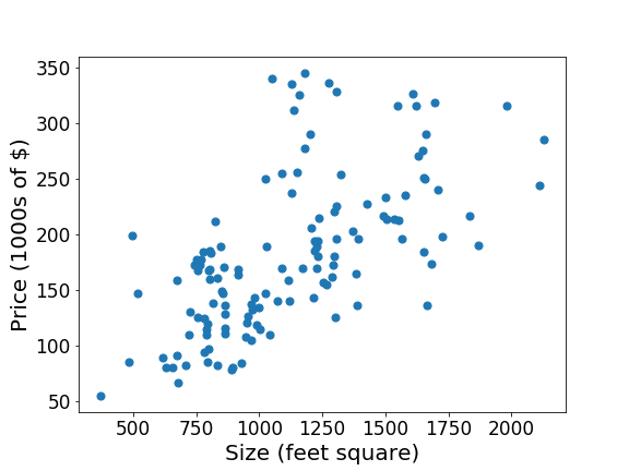
House price prediction
Supervised learning
Given the “right answer” for each example in the data
Regression: Predict a real-valued output
Classification: discrete-valued output
Houston prices:
Training set
| Size | Price |
|---|---|
| 920 | 223 |
| 1060 | 154 |
| 520 | 68 |
| 955 | 127 |
| 902 | 140 |
| ... | ... |
\( x \)
\( y \)
Notation:
\( n \) = Number of training examples
\( x \) = "input" variable / features
\( y \) = "output" variable / "target" variable
Examples:
\( x_1 = 920 \)
\( y_3 = 68 \)
\( (x_4, y_4) = (955, 127) \)
Hypothesis
Training set
Learning algorithm
h
Size of house
Estimated price
Hypothesis
Training set
Learning algorithm
h
Size of house
Estimated price
Hypothesis
Maps \( x \) to \( y \)
\( x \)
Estimated value of \( y \)
How do we represent \( h \)?

\( h(x) = \theta_0 + \theta_1 x \)
Linear regression with one variable
\( \theta \) is called parameters
\( h(x) = \theta_0 + \theta_1 x \)
Cost function
Summary
| x | y |
|---|---|
| 920 | 223 |
| 1060 | 154 |
| 520 | 68 |
| 955 | 127 |
| 902 | 140 |
| ... | ... |
Training set
Hypothesis:
\( h(x) = \theta_0 + \theta_1 x \)
Question:
How to choose the parameters \( \theta_i \)?
\( h(x) = \theta_0 + \theta_1 x \)
\( \theta_0 = 1.5, \theta_1 = 0 \)
\( \theta_0 = 0, \theta_1 = 0.5 \)
\( \theta_0 = 1, \theta_1 = 0.5 \)
\( h(x) \)
\( h(x) = 1.5 + 0 x \)
\( h(x) = 0.5 x \)
Cost function: Intuition
\( x \)
\( y \)
The left one is obviously the best, but why?
\( h(x) \)
\( x \)
\( y \)
\( h(x) \)
Cost function: Intuition
\( x \)
\( y \)
Idea: Choose \( \theta_0, \theta_1 \) so that \( h(x) \) is close to \( y \) for the training examples \( (x, y) \)
\( h(x) \)
\( x \)
\( y \)
\( h(x) \)
Cost function: Intuition
\( x \)
\( y \)
Idea: Choose \( \theta_0, \theta_1 \) so that \( h(x) \) is close to \( y \) for the training examples \( (x, y) \)
\( h(x) \)
\( x \)
\( y \)
\( h(x) \)
Cost function: Intuition
\( x \)
\( y \)
Idea: Choose \( \theta_0, \theta_1 \) so that \( h(x) \) is close to \( y \) for the training examples \( (x, y) \)
\( h(x) \)
J(\theta_0, \theta_1) = \frac{1}{n}
\displaystyle\sum_{i=1}^{n} (h(x_i) - y_i)^2
Cost function: Intuition
\( x \)
\( y \)
Idea: Choose \( \theta_0, \theta_1 \) so that \( h(x) \) is close to \( y \) for the training examples \( (x, y) \)
\( h(x) \)
J(\theta_0, \theta_1) = \frac{1}{n}
\displaystyle\sum_{i=1}^{n} (h(x_i) - y_i)^2
$$ \min_{\theta_0, \theta_1} J(\theta_0, \theta_1) $$
Objective:
Understanding the cost function
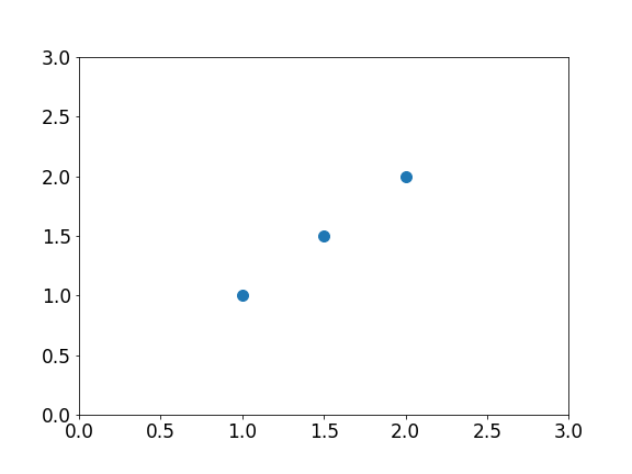
Let's simplify
$$ \min_{\theta_1} J(\theta_1) $$
J(\theta_1) = \frac{1}{n}
\displaystyle\sum_{i=1}^{n} (h(x_i) - y_i)^2
h(x) = \theta_1 x
| x | y |
|---|---|
| 1 | 1 |
| 1.5 | 1.5 |
| 2 | 2 |
Training set
h(x) = \theta_1 x
J(\theta_1)
J(\theta_1)
\theta_1
y
x
h(x) = \theta_1 x
J(\theta_1)
J(\theta_1)
\theta_1
y
x
\theta_1 = 1
h(x) = x
h(x) = \theta_1 x
J(\theta_1)
J(\theta_1)
\theta_1
y
x
\theta_1 = 1
h(x) = x
J(\theta_1) = \frac{1}{3}
\displaystyle\sum_{i=1}^{3} (h(x_i) - y_i)^2
= \frac{1}{3}
(0^2 + 0^2 + 0^2) = 0
h(x) = \theta_1 x
J(\theta_1)
J(\theta_1)
\theta_1
y
x
\theta_1 = 0.5
h(x) = 0.5 x
J(\theta_1) = \frac{1}{3}
((0.5 - 1)^2 + (0.75 - 1.5)^2 + (1 - 2)^2)
= 1.8125
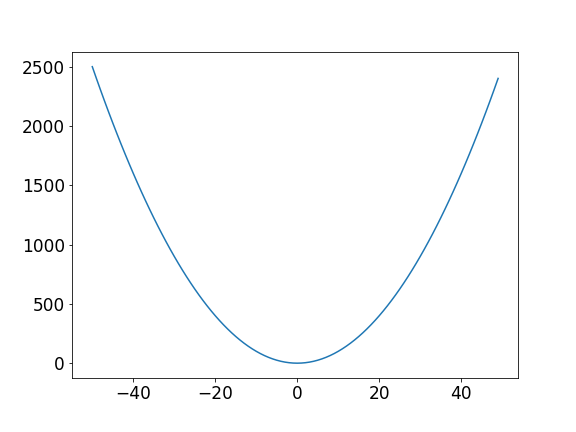
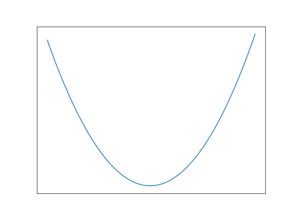
How the cost function might look like
(If you are lucky)
\theta_1
y
J(\theta_1)
\theta_1
The goal
Find the global minimum
\theta_1
y
J(\theta_1)
\theta_1
In 3D
\theta_1
y
J(\theta_1)
\theta_1
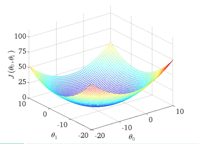
$$ \min_{\theta_0, \theta_1} J(\theta_0, \theta_1) $$
If we consider \( J(\theta_0, \theta_1) \) and want
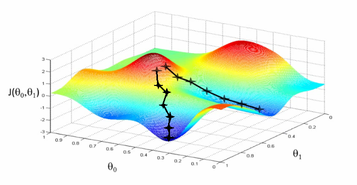
But it also might look like this:
\theta_1
y
J(\theta_1)
\theta_1
Gradient Descent
Summary
Have some function:
Want
Outline:
- Start with some \( \theta_0, \theta_1 \)
- Keep changing \( \theta_0, \theta_1 \) to reduce \( J(\theta_0, \theta_1) \) until we hopefully end up at a minimum
$$ \min_{\theta_0, \theta_1} J(\theta_0, \theta_1) $$
J(\theta_0, \theta_1) = \frac{1}{n}
\displaystyle\sum_{i=1}^{n} (h(x_i) - y_i)^2
Gradient descent algorithm
repeat until convergence {
}
\theta_j := \theta_j - \alpha \frac{\partial}{\partial \theta_j} J(\theta_0, \theta_1)
\( \partial \) = partial derivative = a derivative of a function of two or more variables with respect to one variable, the other(s) being treated as constant.
Gradient descent algorithm
repeat until convergence {
}
\theta_j := \theta_j - \alpha \frac{\partial}{\partial \theta_j} J(\theta_0, \theta_1)
learning rate
derivative
Gradient descent algorithm
repeat until convergence {
}
\theta_j := \theta_j - \alpha \frac{\partial}{\partial \theta_j} J(\theta_0, \theta_1)
"Size of the step"
"One step deeper" or "Direction of the step"
Gradient descent
In our case
repeat until convergence {
}
\theta_0 := \theta_0 - \alpha \frac{\partial}{\partial \theta_0} J(\theta_0, \theta_1)
\theta_1 := \theta_1 - \alpha \frac{\partial}{\partial \theta_1} J(\theta_0, \theta_1)
Simultaneous
Visual representation
\theta_1
J(\theta_1)
Visual representation
\theta_1
Tangent of \( \theta_1 \)
Derivative \( \approx \) Step in the tangent direction
Visual representation
\theta_1
\theta_1 - \alpha \frac{\partial}{\partial \theta_1} J(\theta_1)
Visual representation
Minimum found!
If \( \alpha \) is too small, the gradient descent can be slow
If \( \alpha \) is too large, gradient descent can overshoot the minimum. It may fail to converge or even diverge.
Local and global minimum
Gradient descent give no assurance if we reach a global minimum

What we learned today
Our first supervised model with the hypothesis:
\( h(x) = \theta_0 + \theta_1 x \)
We have a function ("cost function") to evaluate this model error:
And an algorithm to minimize this function in order to get the best parameters \( \theta_0, \theta_1 \):
Repeat until convergence {
}
J(\theta_0, \theta_1) = \frac{1}{n}
\displaystyle\sum_{i=1}^{n} (h(x_i) - y_i)^2
\theta_j := \theta_j - \alpha \frac{\partial}{\partial \theta_j} J(\theta_0, \theta_1)
Data Science 101.1
By ycarbonne


