\begin{Bmatrix}
雙擺運動\\
_{以不同力學方式分析}
\end{Bmatrix}
組員:11張秉諺 16 陳亮延 24 楊書桓 29蔡政廷
第一組
1
研究動機
2
研究摘要
3
文獻探討
5
實驗結果
4
研究方法
6
參考資料
# 1.研究動機
研究動機
在指定作業3-2中,我們以傳統牛頓力學方式及力學能守恆分析雙擺的受力並模擬運動情形,所以我們在想能不能以方式(廣義座標、廣義速度、能量)分析其力學,並且模擬出其運動情形,最後比較其差異。


# 2.研究摘要
研究摘要
以拉格朗日力學用能量的觀點推導出雙擺運動中兩顆球體的角加速度,並用角加速度算出每個時刻的位置與速度,觀察以拉格朗日力學模擬的雙擺運動是否運作得比牛頓力學模擬的程式順暢,並觀察是否與牛頓力學分析的結果一致。

文獻探討
拉格朗日力學
笛卡爾座標系與廣義坐標系
文獻探討:拉格朗日力學
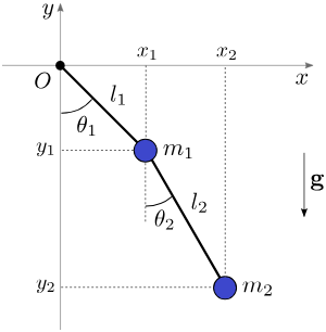
單就雙擺系統而言,
在笛卡爾座標系中我們會以四個參數\((x_1,y_1,x_2,y_2)\)表示其座標。
然而每個座標之間擁有約束(有關),並不能自由存在這個平面上,
透過求自由度,可以知道表達這個系統所需的最小座標數。
以雙擺系統來說,其自由度為2,
也就是兩個參數即可表示當前系統位置狀態,
這兩個參數即\((\theta_1\theta_2)\),此時:
x_1=l_1\sin\theta_1\\
x_2=l_1\sin\theta_1
\begin{aligned}
&y_1=-l_1\cos\theta_1\\
&y_2=-l_1\cos\theta_1-l_2\cos\theta_2
\end{aligned}
拉格朗日量(拉格朗日函數)
拉格朗日力學中,我們得引入一個拉格朗日量(函數)
以進行拉格朗日方程式的運算,其定義為:\(L=E_k-U\)
而在雙擺系統中,經計算,我們可以這樣表示:
\begin{aligned}
E_k=&\frac{1}{2}m_1v_1^2+\frac{1}{2}m_2v_2^2\\
=&\frac{1}{2}m_1(\dot{x}_1^2+\dot{y}_1^2)+\frac{1}{2}m_2(\dot{x}_2^2+\dot{y}_2^2)\\
=&\frac{1}{2}m_1 l_1^2 \dot{\theta}_1^2 + \dfrac{1}{2}m_2[ l_1^2 \dot{\theta}_1^2+ l_2^2 \dot{\theta}_2^2
+ 2l_1l_2\dot{\theta}_1\dot{\theta}_2\cos(\theta_1-\theta_2)]\\
U=&m_1gy_1+m_2gy_2\\
=&-m_1gl_1\cos\theta_1-m_2g(l_1\cos\theta_1+l_2\cos\theta_2)\\
=&-(m_1+m_2)gl_1\cos\theta_1-m_2gl_2\cos\theta_2\\
L=&\frac{1}{2}(m_1+m_2)l_1^2\dot{\theta}_1^2+\frac{1}{2}m_2l_2^2\dot{\theta}_2^2+m_2l_1l_2\dot{\theta}_1\dot{\theta}_2\cos(\theta_1-\theta_2)\\
&+(m_1+m_2)gl_1\cos \theta_1+m_2gl_2\cos\theta_2
\end{aligned}
※\(\dot{a}\)為a函式對t微分
文獻探討:拉格朗日力學
拉格朗日方程式
計算完拉格朗日量後,我們便可透過拉格朗日方程式求出運動方程式。
拉格朗日方程如下:\(\displaystyle\frac{d}{dt}\frac{\partial L}{\partial \dot{q}_i}-\frac{\partial L}{\partial q_i}=Q_1\)
\(q_i\)是為廣義座標,\(Q_i\)則為非保守力,
\(\displaystyle\frac{d}{dt}\)為對時間微分,\(\displaystyle \frac{\partial}{\partial x}\)則為對x偏微分
雙擺運動中,
系統不受非保守外力,因此\(Q_i=0\),故得出:
\begin{aligned}
\begin{cases}
(m_1+m_2)l_1\ddot\theta_1+m_2l_2\ddot\theta_2\cos(\theta_1-\theta_2)+m_2l_2\dot\theta_2^2\sin(\theta_1-\theta_2)+(m_1+m_2)g\sin\theta_1&=0\\
l_2\ddot\theta_2+l_1\ddot\theta\cos(\theta_1-\theta_2)-l_1\dot\theta_1^2\sin(\theta_1-\theta_2)+g\sin\theta_2&=0
\end{cases}
\end{aligned}
文獻探討:拉格朗日力學
拉格朗日方程式
\begin{aligned}
\begin{cases}
(m_1+m_2)l_1\ddot\theta_1+m_2l_2\ddot\theta_2\cos(\theta_1-\theta_2)+m_2l_2\dot\theta_2^2\sin(\theta_1-\theta_2)+(m_1+m_2)g\sin\theta_1&=0\ (1)\\
l_2\ddot\theta_2+l_1\ddot\theta\cos(\theta_1-\theta_2)-l_1\dot\theta_1^2\sin(\theta_1-\theta_2)+g\sin\theta_2&=0\ (2)
\end{cases}
\end{aligned}
文獻探討:拉格朗日力學
由於這個算式過於複雜,
所以我們可以用幾個函數去簡化表示它:
\begin{aligned}
\alpha_1(\theta_1,\theta_2)&=\frac{l_2}{l_1}(\frac{m_2}{m_1+m_2})\cos(\theta_1-\theta_2)\\
\alpha_2(\theta_1,\theta_2)&=\frac{l_1}{l_2}\cos(\theta_1-\theta_2)
\end{aligned}
\begin{aligned}
f_1(\theta_1,\theta_2,\dot{\theta_1},\dot{\theta_2})&=-\frac{m_2}{m_1+m_2}\dot{\theta_2}^2\sin(\theta_1-\theta_2)-\frac{g}{l_1}\sin\theta_1\\
f_2(\theta_1,\theta_2,\dot{\theta_1},\dot{\theta_2})&=\frac{l_1}{l_2}\dot\theta_1^2\sin(\theta_1-\theta_2)-\frac{g}{l_2}\sin\theta_2
\end{aligned}
\Rightarrow
\begin{cases}
\ddot\theta_1+\alpha_1(\theta_1,\theta_2)\ddot\theta_2=f_1(\theta_1,\theta_2,\dot{\theta_1},\dot{\theta_2})\ (3)\\
\ddot\theta_2+\alpha_2(\theta_1,\theta_2)\ddot\theta_1=f_2(\theta_1,\theta_2,\dot{\theta_1},\dot{\theta_2})\ (4)
\end{cases}
拉格朗日方程式
\begin{aligned}
\begin{cases}
(m_1+m_2)l_1\ddot\theta_1+m_2l_2\ddot\theta_2\cos(\theta_1-\theta_2)+m_2l_2\dot\theta_2^2\sin(\theta_1-\theta_2)+(m_1+m_2)g\sin\theta_1&=0\ (1)\\
l_2\ddot\theta_2+l_1\ddot\theta\cos(\theta_1-\theta_2)-l_1\dot\theta_1^2\sin(\theta_1-\theta_2)+g\sin\theta_2&=0\ (2)
\end{cases}
\end{aligned}
文獻探討:拉格朗日力學
\Rightarrow
\begin{cases}
\ddot\theta_1+\alpha_1(\theta_1,\theta_2)\ddot\theta_2=f_1(\theta_1,\theta_2,\dot{\theta_1},\dot{\theta_2})\ (3)\\
\ddot\theta_2+\alpha_2(\theta_1,\theta_2)\ddot\theta_1=f_2(\theta_1,\theta_2,\dot{\theta_1},\dot{\theta_2})\ (4)
\end{cases}
我們可以再以矩陣來表示這個等式:
A\begin{bmatrix}
\ddot\theta_1\\
\ddot\theta_2
\end{bmatrix}
=
\begin{bmatrix}
1&\alpha_1\\
\alpha_2&1
\end{bmatrix}
\begin{bmatrix}
\ddot\theta_1\\
\ddot\theta_2
\end{bmatrix}
=
\begin{bmatrix}
f_1\\f_2
\end{bmatrix}
再計算\(A\)的反方陣,便可求出兩角加速度\((\ddot\theta_1,\ddot\theta_2)\):
\begin{aligned}
A^{-1} &=
\displaystyle\frac{1}{\det(A)}
\begin{bmatrix}
1 & -\alpha_1 \\
-\alpha_2 & 1
\end{bmatrix}
=
\displaystyle\frac{1}{1 - \alpha_1\alpha_2}
\begin{bmatrix}
1 & -\alpha_1 \\
-\alpha_2 & 1
\end{bmatrix}
\\
&\Rightarrow
\begin{bmatrix}
\ddot{\theta}_1 \\ \ddot{\theta}_2 \end{bmatrix}=
A^{-1}
\begin{bmatrix} f_1 \\[3pt] f_2 \end{bmatrix}
=
\displaystyle\frac{1}{1 - \alpha_1\alpha_2}
\begin{bmatrix} f_1 - \alpha_1 f_2\\[3pt] -\alpha_2 f_1 + f_2 \end{bmatrix}\ (5)
\end{aligned}
拉格朗日方程式
\begin{aligned}
\begin{cases}
(m_1+m_2)l_1\ddot\theta_1+m_2l_2\ddot\theta_2\cos(\theta_1-\theta_2)+m_2l_2\dot\theta_2^2\sin(\theta_1-\theta_2)+(m_1+m_2)g\sin\theta_1&=0\ (1)\\
l_2\ddot\theta_2+l_1\ddot\theta\cos(\theta_1-\theta_2)-l_1\dot\theta_1^2\sin(\theta_1-\theta_2)+g\sin\theta_2&=0\ (2)
\end{cases}
\end{aligned}
文獻探討:拉格朗日力學
\Rightarrow
\begin{cases}
\ddot\theta_1+\alpha_1(\theta_1,\theta_2)\ddot\theta_2=f_1(\theta_1,\theta_2,\dot{\theta_1},\dot{\theta_2})\ (3)\\
\ddot\theta_2+\alpha_2(\theta_1,\theta_2)\ddot\theta_1=f_2(\theta_1,\theta_2,\dot{\theta_1},\dot{\theta_2})\ (4)
\end{cases}
\begin{aligned}
A^{-1} &=
\displaystyle\frac{1}{\det(A)}
\begin{bmatrix}
1 & -\alpha_1 \\
-\alpha_2 & 1
\end{bmatrix}
=
\displaystyle\frac{1}{1 - \alpha_1\alpha_2}
\begin{bmatrix}
1 & -\alpha_1 \\
-\alpha_2 & 1
\end{bmatrix}
\\
&\Rightarrow
\begin{bmatrix}
\ddot{\theta}_1 \\ \ddot{\theta}_2 \end{bmatrix}=
A^{-1}
\begin{bmatrix} f_1 \\[3pt] f_2 \end{bmatrix}
=
\displaystyle\frac{1}{1 - \alpha_1\alpha_2}
\begin{bmatrix} f_1 - \alpha_1 f_2\\[3pt] -\alpha_2 f_1 + f_2 \end{bmatrix}\ (5)
\end{aligned}
如此一來便可求得角加速度,
便能輕易運算下一秒的廣義座標,進而得出位置了!
研究方式
以拉格朗日力學模擬的雙擺系統
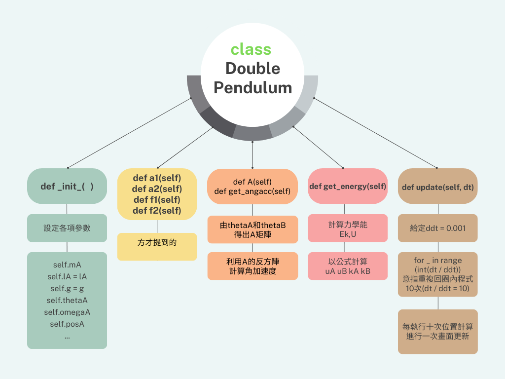
class DoublePendulum
給定各項參數使其模組化
self.mA
self.g = g
self.thetaA
......
1.
def _init_
\(\alpha_1,\alpha_2\\f_1,f_2\)
2.
def a1,a2,f1,f2
由\(\theta_1\)和\(\theta_2\)得出A矩陣,最後利用A矩陣的反矩陣求角加速度
3.
def A(self)
def get_angacc(self)
研究方法:以拉格朗日力學模擬的雙擺系統
以公式計算
uA
uB
kA
kB
4.
def get_energy
dt為自定義變數,決定其畫面更新率,ddt為程式運作的速度
5.
def update
研究方法:以拉格朗日力學模擬的雙擺系統
class DoublePendulum
研究方法:以拉格朗日力學模擬的雙擺系統
class DoublePendulum
\alpha_1,\alpha_2,f_1,f_2
3-2基本寫法(牛頓力學)
import numpy as np

def spring_force(k, r, x0):
    return -k * (np.linalg.norm(r) - x0) * r / np.linalg.norm(r)

class DoublePendulum:
    def __init__(self, mA, mB, lA, lB, g, thetaA, thetaB):
        self.mA = mA
        self.mB = mB
        self.lA = lA
        self.lB = lB
        self.g = g
        self.posA = np.array([lA*np.sin(thetaA), -lA*np.cos(thetaA), 0])
        self.posB = self.posA + np.array([lB*np.sin(thetaB), -lB*np.cos(thetaB), 0])
        self.velA = np.array([0.0, 0.0, 0.0])
        self.velB = np.array([0.0, 0.0, 0.0])

    def get_energy(self):
        uA = self.mA * self.g * self.posA[1]
        uB = self.mB * self.g * self.posB[1]
        kA = 0.5 * self.mA * np.dot(self.velA, self.velA)
        kB = 0.5 * self.mA * np.dot(self.velB, self.velB)
        return uA+uB, kA+kB, uA+uB+kA+kB

    def update(self, dt):
        ddt = 0.0001
        k = 100000
        for _ in range(int(dt / ddt)):
            aA = (np.array([0, -self.mA * self.g, 0]) + spring_force(k, self.posA, self.lA) - spring_force(k, self.posB - self.posA, self.lB)) / self.mA
            aB = (np.array([0, -self.mB * self.g, 0]) + spring_force(k, self.posB - self.posA, self.lB)) / self.mB
            self.velA += aA*ddt
            self.velB += aB*ddt
            self.posA += self.velA*ddt
            self.posB += self.velB*ddt
研究方法:以拉格朗日力學模擬的雙擺系統
自訂函式庫
import numpy as np

class DoublePendulum:#以class貯存函式庫
    def __init__(self, mA, mB, lA, lB, g, thetaA, thetaB):#參數設定
        self.mA = mA
        self.mB = mB
        self.lA = lA
        self.lB = lB
        self.g = g
        self.thetaA = thetaA
        self.thetaB = thetaB
        self.omegaA = 0
        self.omegaB = 0

    def a1(self):
        return (self.lB / self.lA) * (self.mB / (self.mA + self.mB)) * np.cos(self.thetaA - self.thetaB)

    def a2(self):
        return (self.lA / self.lB) * np.cos(self.thetaA - self.thetaB)

    def f1(self):
        return -(self.lB / self.lA) * (self.mB / (self.mA + self.mB)) * self.omegaB**2 * np.sin(self.thetaA - self.thetaB) - (self.g / self.lA) * np.sin(self.thetaA)

    def f2(self):
        return (self.lA / self.lB) * self.omegaA**2 * np.sin(self.thetaA - self.thetaB) - (self.g / self.lB) * np.sin(self.thetaB)

    def A(self):
        return np.array([[1, self.a1()], [self.a2(), 1]])

    def get_angacc(self): #計算角加速度
        v = np.array([self.f1(), self.f2()])
        invA = np.linalg.inv(self.A())
        return np.dot(invA, v)

    def get_energy(self): #計算力學能
        uA = -self.mA * self.g * self.lA * np.cos(self.thetaA)
        uB = -self.mB * self.g * (self.lA*np.cos(self.thetaA) + self.lB*np.cos(self.thetaB))
        kA = (1/2) * self.mA * (self.lA * self.omegaA)**2
        vB = np.array([
            self.omegaA * self.lA * np.cos(self.thetaA) + self.omegaB * self.lB * np.cos(self.thetaB),
            self.omegaA * self.lA * np.sin(self.thetaA) + self.omegaB * self.lB * np.sin(self.thetaB)
        ])
        kB = (1/2) * self.mB * np.dot(vB, vB)
        return uA+uB, kA+kB, uA+uB+kA+kB

    def update(self, dt): #更新畫面
        ddt = 0.001 #程式更新速度
        for _ in range(int(dt / ddt)):
            angacc = self.get_angacc()
            self.thetaA += self.omegaA * ddt
            self.thetaB += self.omegaB * ddt
            self.omegaA += angacc[0] * ddt
            self.omegaB += angacc[1] * ddt
研究方法:以拉格朗日力學模擬的雙擺系統
引用vpython模組畫圖
import lagrangian
import newtonian
from vpython import *

def np_to_vpy(nparr):
    return vector(nparr[0], nparr[1], nparr[2])

class Renderer:
    def __init__(self, pendulums):
        self.pendulums = pendulums
        self.comps = []
        for _ in pendulums:
            components = {
                'ballA': sphere(radius=1, pos=vector(0, 0, 0)),
                'ballB': sphere(radius=1, pos=vector(0, 0, 0), make_trail=False),
                'rodA': cylinder(radius=0.1, pos=vector(0, 0, 0)),
                'rodB': cylinder(radius=0.1, pos=vector(0, 0, 0)),
                'graph': graph(width=640, height=640, align='left'),
                'ucurve': gcurve(color=color.red),
                'kcurve': gcurve(color=color.blue),
                'ecurve': gcurve(color=color.black)
            }
            self.comps.append(components)

    def draw(self, i, offset, color):
        self.comps[i]['ballA'].color = color
        self.comps[i]['ballB'].color = color

        self.comps[i]['ballA'].pos = np_to_vpy(self.pendulums[i].posA) + offset
        self.comps[i]['ballB'].pos = np_to_vpy(self.pendulums[i].posB) + offset
        self.comps[i]['ballB'].make_trail = True

        self.comps[i]['rodA'].pos = offset
        self.comps[i]['rodA'].axis = self.comps[i]['ballA'].pos - offset
        self.comps[i]['rodB'].pos = self.comps[i]['ballA'].pos
        self.comps[i]['rodB'].axis = self.comps[i]['ballB'].pos - self.comps[i]['ballA'].pos

    def graph(self, i, t):
        u, k, e = self.pendulums[i].get_energy()
        self.comps[i]['ucurve'].plot(pos=(t, u))
        self.comps[i]['kcurve'].plot(pos=(t, k))
        self.comps[i]['ecurve'].plot(pos=(t, e))

if __name__ == '__main__':
    lA = 10
    lB = 10
    dplag = lagrangian.DoublePendulum(1, 1, lA, lB, 9.8, (1/2)*pi, (1/2)*pi)
    dpnew = newtonian.DoublePendulum(1, 1, lA, lB, 9.8, (1/2)*pi, (1/2)*pi)
    scene = canvas(
        width=1280, height=720,
        center=vector(0, 0, 0)
    )
    rend = Renderer([dplag, dpnew])
    t = 0
    dt = 0.05
    while True:
        rate(24)

        rend.draw(0, vector(-20, 0, 0), color.cyan)
        rend.draw(1, vector(20, 0, 0), color.yellow)
        rend.graph(0, t)
        rend.graph(1, t)
        dplag.update(dt)
        dpnew.update(dt)

        t += dt
研究方法:以拉格朗日力學模擬的雙擺系統
實驗結果
以拉格朗日力學模擬的雙擺系統
參考資料
#參考資料-拉格朗日力學
參考資料
wikipedia(2023 年 6 月 11 日)。Lagrangian mechanics。Wikipedia The Free Encyclopedia 。 https://en.wikipedia.org/wiki/Lagrangian_mechanics
Diego Assencio(2014 年 2 月 28 日)。The double pendulum: Lagrangian formulation。diego.assencio.com。 https://diego.assencio.com/?index=1500c66ae7ab27bb0106467c68feebc6
分工比例
張秉諺:22%
陳亮延:26%
楊書桓:22%
蔡政廷:30%
Code
By YEN


