Algebraic Geometry:
Computing with polynomials
What is covered:
- Definitions and concepts
- Common problems
- Basic algorithms
What isn't covered:
- State of the art algorithms and heuristics
- Correctness and proofs in general
- Tools and case studies
Introductory talk!
Sources: Papers, books, presentations - if you need more, ask...
(Univariate) Polynomial
Expression of constants, one variable, multiplication, addition and positive constant exponentiation:
p(x) = a_n x^n + a_{n-1} x^{n-1} + ... + a_1 x + a_0
- coefficients are members of (some) ring
- degree n (zero for constant polynomial but undefined for zero polynomial)
- polynomials form a ring (we can do factorisation)
- at most n real roots (solutions of p(x) = 0)
- In general, we assume rational coefficients
- Rational roots can be found using factorisation
- Real roots of polynomials can be expressed explicitly for n < 5 (discriminant, etc.)
- For n >= 5, we don't have an algorithm to find the exact algebraic expression, but we can still check if/where the root exists
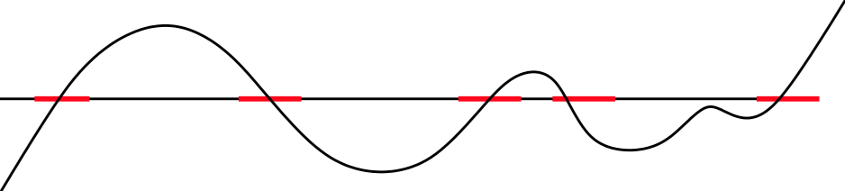
Root Isolation
Isolation problem: Given a polynomial, compute rational intervals such that each interval contains exactly one root and each root is covered by some interval.
How do you compute this?
Descartes rule of signs (1637)
\text{Number of real roots of } p(x) \text{ where } x \in (0, \infty{}) \\ \text{ is at most the sign change number of sequence } a_n, \ldots, a_0; \\ \text{ Both numbers have the same parity }
Corollary:
no sign changes = no root; one sign change = one root
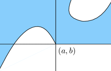
Verify that interval (a, b) isolates exactly one root: "stretch" the interval across positive numbers.
(b - x)^n \cdot p(\frac{x-a}{b-x})
How do you compute this?
Full algorithm:
- Start with interval (-M, M)
- "Stretch" to positive numbers
- Compute sign changes
- If zero, skip;
- If one, output isolating interval;
- If >1, divide interval and continue recursively.
M = max_i\ 2 \cdot \frac{a_i}{a_n}
- Polynomial in both degree and coefficient bit size
- Can be extended to polynomials with real coefficients
- Faster (smaller polynomial) algorithms exist: Pan's algorithm
Real Algebraic Numbers
Real numbers which can be expressed
as roots of a polynomial.
Representation: Polynomial + isolating interval
Can be manipulated "efficiently" (addition, multiplication, etc.)
Form a ring => can be used as polynomial coefficients! (and root isolation still works)
Multivariete Polynomial
Two views:
- Multiple variables: x, y, z, ...
- Univariate polynomial with polynomial coefficients
Most interesting problems assume multiple variables :(
(ax^2 + bx + c)y^2 + (dx^5 + \ldots + e)y + \ldots
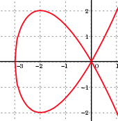
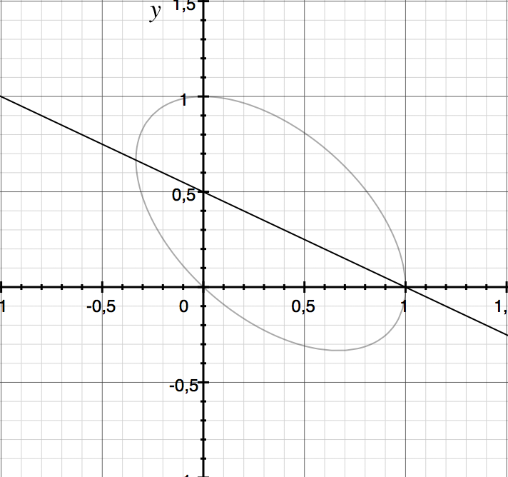
Algebraic curve: p(x, y) = 0
Tarski sentence: A quantified formula over polynomial inequalities
Algebraic variety (or set): all given multivariate polynomials are zero
Semi-algebraic set: all given multivariate polynomial inequalities are satisfied
\forall x. \exists y. (x^2 - y \geq 0 \land x - y + 1 < 0)
Problems:
-
Membership
-
Emptiness/Sample points
-
Intersection/union/etc.
-
Variable/quantifier elimination
-
Projection
-
Visualisation
Resultant
Expression of coefficients of polynomials p and q which is 0 iff the two polynomials have a common root.
Res[(x^2-x-2), (x-4)(x-1)] = 0
Res[(x^2-x-2), (x-2)(x-1)] = 1
Subresultants
i-th subresultant: expression of coefficients of polynomials p and q which is 0 iff the two polynomials have a common root of multiplicity i.
SRes_3[(x^2-x-2)^2, (x-2)^2(x-1)] = 0
SRes_2[(x^2-x-2)^2, (x-2)^2(x-1)] = 4
How do you compute this?
Sylvester matrix:
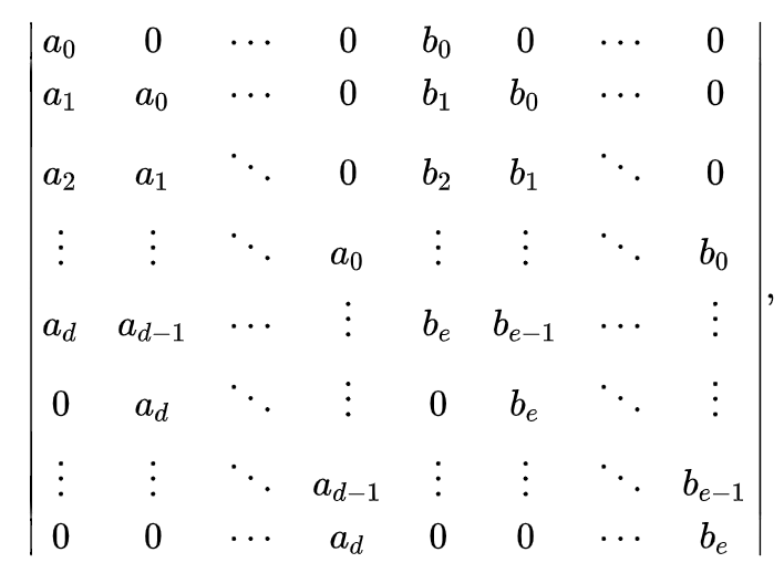
Resultant is the determinant, subresultants are determinants of various sub-matrices.
Why does it work?

We can extend this to multiple variables!
K-variable polynomials P and Q are just univariate polynomials in a ring of (k-1)-variable polynomials.
Matrix of coefficients = Matrix of polynomials
Determinant = (k-1)-variable polynomial S
Properties still hold: S is zero if and only if both P and Q are zero, but has one less variable!
Wait, what just happened?!
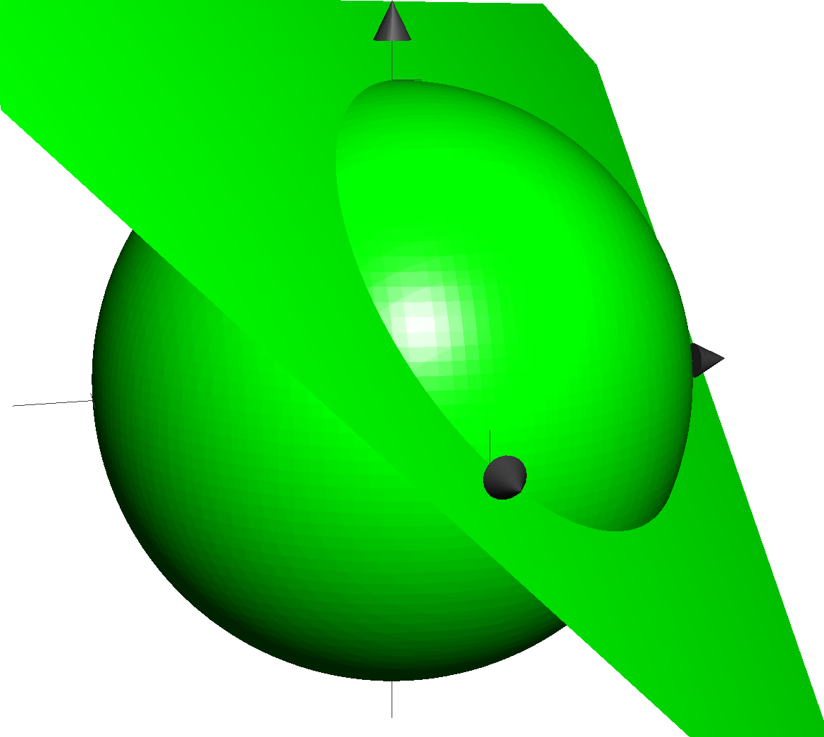
Projection!

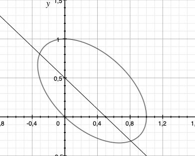
x^2+y^2+z^2-1 = 0 \\ x+y+z-1 = 0
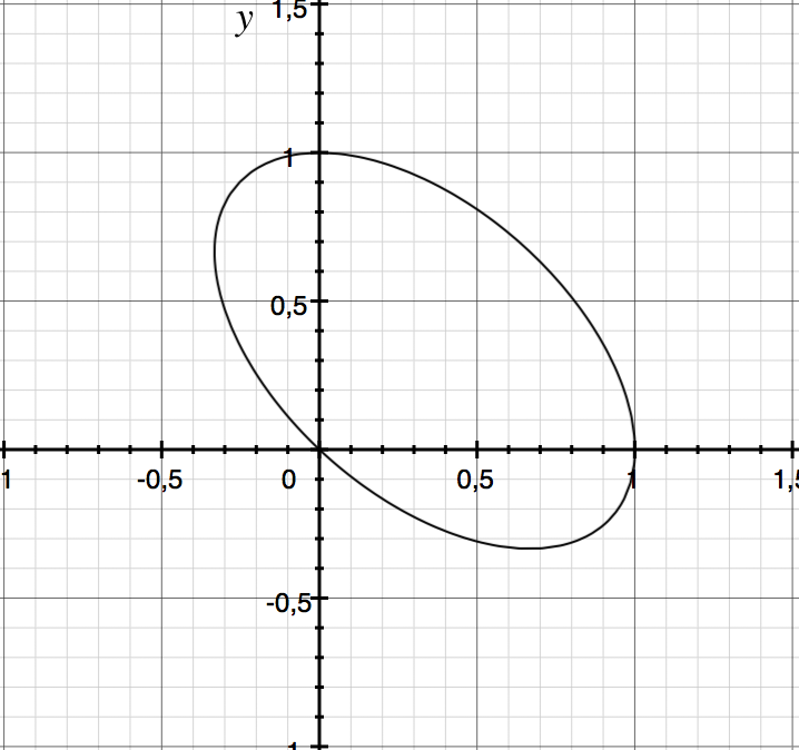
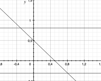
x^2 + xy - x + y^2 - y = 0
x^2 + xy - x + y^2 - y = 0 \\ x + 2y - 1 = 0\ (\frac{df}{dy})
3x^2 - 2x - 1 = 0
(discriminant)
Complexity of naively computing determinants is not exactly great :(
Dimensionality is not free: Projection from n to 1 dimension yields exponentially larger resultant polynomial in the worst case.
However, polynomials are a symbolic representation: in many cases, the result need not be exponentially larger.
Also, subresultants are usually used in practice, because they can be smaller. If roots with high multiplicities exist, subresultans can give answer much faster.
Thankfully, other efficient algorithms exist (cubic in the number of coefficient operations).
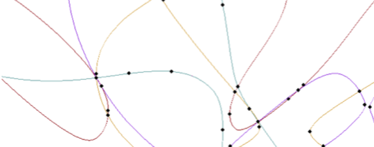
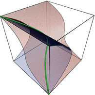
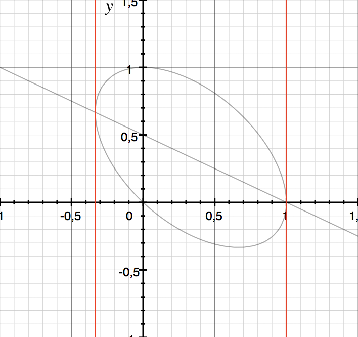
Cyllindrical Algebraic Decomposition
Divide the space into sign-invariant connected regions. For each region, provide a sample point.
Idea: Using projection, ensure intersections, self-intersections and folds are preserved into lower dimensions:
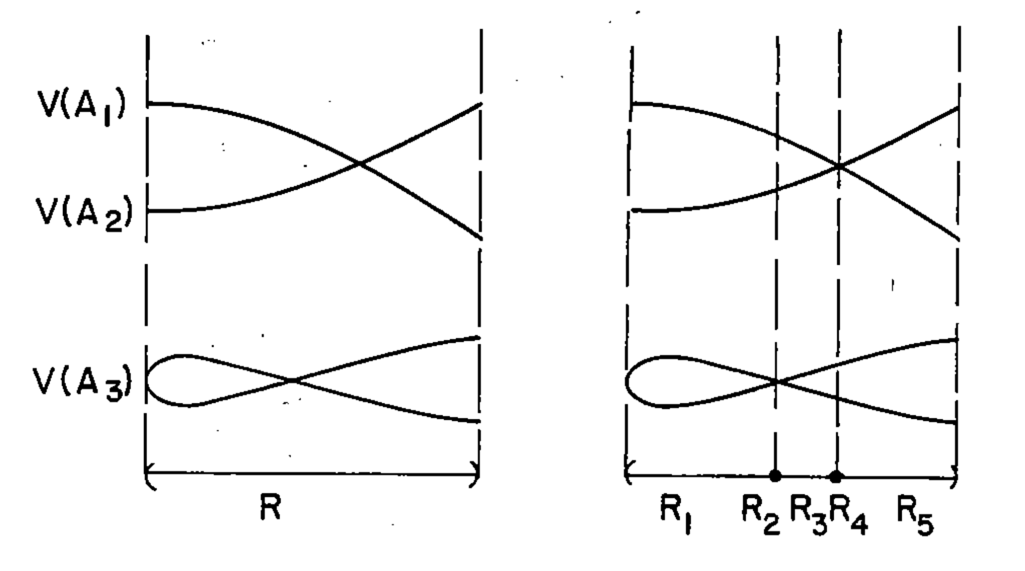
Algorithm overview:
Idea: Reduce to 1-dimensional problem. N-dimensional CAD can be then extended to (n+1)-dimensional.
- Recursively compute determinants of each polynomial and pairwise resultants until univariate;
- Isolate roots of the resulting polynomials => 1D CAD;
- Expand each cell of n-D CAD to a (n+1)-D cyllinder.
Expansion of cell:
- Substitute the n-D sample point into the (n+1)-D polynomials => result are 1D polynomials;
- Isolate roots => 1D CAD;
- Extend the n-D sample point with each sample point from the new 1D CAD.
CAD can be used to solve essantially anything regarding polynomials, but is also very costly: doubly-exponential in the number of dimensions;
Simplifications:
- CAD where only n (or n-1) dimensional cells are computed (lower dimensions are discarded) - exponential;
- Bounded CAD: heuristics can eliminate polynomials which are already sign invariant in the bounded region; cell expansion is also simplified.
Can we go faster for simpler problems?
Groebner Basis
Ideal (simplified): Given a set of polynomials, ideal is the algebraic structure formed by multiplying these polynomials with other arbitrary polynomials.
Corollary: If two sets of polynomials generate the same ideal, they have the same zeroes (vanishing points).
Groebner basis: A canonical set of generating polynomials for a given ideal. (Canonical up to monomial order)
Algorithm idea: Based on gaussian elimination for linear systems, but each monomial is substituted with a new variable.
Problem: Requires as many equations as monomials. Needs to be "padded" appropriately to work.
Various monomial orderings can have vastly different complexity!
Elimination order: Eliminates variables, similar to resultants, similar complexity.
Test for emptiness and equality of ideals works with any ordering. (Emptiness = solution to system of equations)
Groebner basis can be vastly simpler than the original ideal:
x^2 + xy - x + y^2 - y\\
2x + 2y - 1
4y^2 -2y -1\\
2x + 2y - 1
Applications...
Algebraic Geometry:
By Samuel Pastva


