Finding (bottom) SCCs in many systems at once using symbolic algorithms
Samuel Pastva
A gentle reminder that we should not forget this is still happening...
Motivation
Logical Modelling in Systems Biology
Boolean Network
f_1(x) = x_1 \land x_2
f_2(x) = \neg x_1 \lor x_3
f_3(x) = (x_1 \land x_2) \lor (\neg x_1 \land \neg x_3)
n Boolean variables—genes, proteins, other biochemical entities
Update functions—one per variable
Boolean Network (with inputs)
f_1(x, {\color{red} p}) = x_1 \land ({\color{red} p_1} \Rightarrow x_2)
f_2(x, {\color{red} p}) = \neg x_1 \lor (x_3 \land \neg {\color{red} p_1})
f_3(x, {\color{red} p}) = (x_1 \land x_2) \lor (\neg x_1 \land \neg x_3 \land {\color{red} p_2})
m Boolean inputs/constants/parameters—arbitrary but fixed values
Synchronous dynamics
x_{t+1} = f(x_{t}, p)
Asynchronous dynamics
f_1(x_t, p) \mid\mid f_2(x_t, p) \mid\mid f_3(x_t, p)
and others...
What happens to the system eventually?
Bottom/Terminal strongly connected components
(attractors)
Single states, cycles, more complex sets...
Long-lived transients—other non-trivial SCCs
Different input valuations lead to different outcomes
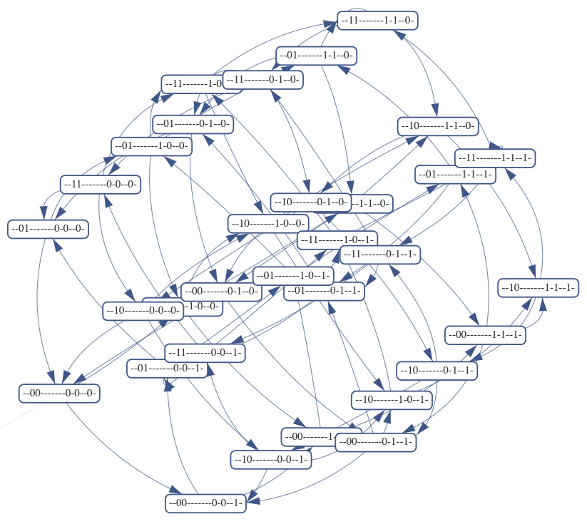
G = (V, C, E)~\text{(coloured graph)}
V = \mathbb{B}^n~\text{(states)}
C = \mathbb{B}^m~\text{(input val.)}
E \subseteq V \times C \times V~\text{(col. edges)}
Typically at least 2^50, often 2^100 or more in total
Symbolic Algorithms
with Binary Decision Diagrams*
*Bryant, Randal E. "Graph-based algorithms for Boolean function manipulation." Computers, IEEE Transactions on 100.8 (1986): 677-691.
| x_1 | x_2 | x_3 |
|---|---|---|
| 1 | 0 | 1 |
| 1 | 0 | 0 |
| 0 | 1 | 1 |
(x_1 \land \overline{x_2}) \lor (\overline{x_1} \land x_2 \land x_3)
Formula is satisfied exactly for valuations from the set
Set of states:
Boolean formula:
x_1
x_2
x_2
x_3
x_3
x_3
x_3
0
0
0
1
1
1
0
0
Binary decision tree:
x_1
x_2
x_2
x_3
x_3
x_3
x_3
0
0
1
1
0
Binary Decision Diagram
x_1
x_2
x_2
x_3
0
1
1
0
Binary Decision Diagram
x_1
x_2
x_2
x_3
0
1
Binary Decision Diagram
Canonical for each Boolean function (assuming fixed variable order)
Often exponentially smaller than the original tree or a DNF formula (not always)
Bit-vector set ~ Boolean formula ~ BDD
(or relation)
Set op. ~ Logical op. ~ Graph op.
O(n^2) in the number of BDD nodes (mostly)
Not the size of the set! (or formula/tree/etc.)
Symbolic complexity model: one unit of work = one BDD operation
Symbolic complexity model is often surprising
\mathcal{O}(n^2)~\text{symbolic operations}
\mathcal{O}(n)~\text{symbolic operations}
\mathcal{O}(n)
\mathcal{O}(n^3)
The first case is "practically" much better!
Nobody can usually give you these bounds...
...but we know
it happens "in the wild":
Reachability with saturation
\texttt{Post} (i, X \subseteq V) = \{ y \in V \mid \exists x \in X.~x \xrightarrow{i} y \}
\text{Successors using a single}~f_i:
\text{Successors using all}~f_i:
\texttt{PostAll} (X \subseteq V) = \bigcup_{i} \texttt{Post}(i, X)
\texttt{Post} (i, X \subseteq V {\color{red} \times C}) = \{ (y, c) \mid \exists (x, c) \in X.~x \xrightarrow{i}_{\color{red} c} y \}
\text{Successors using a single}~f_i:
\text{Successors using all}~f_i:
\texttt{PostAll} (X \subseteq V {\color{red} \times C}) = \bigcup_{i} \texttt{Post}(i, X)
"Normal" reachability
def FWD(initial):
  result = initial
  next = PostAll(initial)
  while next != result:
    result = next
    next = result.union(PostAll(result))
  return result
"Saturation" reachability*
def FWD(initial):
  result = initial
  done = False
  while not done:
    done = True
    for i in [1,n]:
      next = Post(i, result)
      if not next.is_subset(result):
        result = result.union(next)
        done = False
  return result
*Ciardo, Gianfranco, Gerald Lüttgen, and Radu Siminiceanu. "Saturation: an efficient iteration strategy for symbolic state—space generation." International Conference on Tools and Algorithms for the Construction and Analysis of Systems. Springer, Berlin, Heidelberg, 2001.
A simplified case for Boolean variables... more complex domains need extra loop here
"Normal" reachability:
- Asymptotically optimal (linear in the graph diameter)
- Typically out of memory for n>60
"Saturation" reachability:
- Not optimal (O(|V|log(|V|)), but depends)
- Typically makes good progress well into n>100, often n>1000 (depends on relationships between individual update functions)
Symbolic (bottom) SCC computation
(finally)
SCC closed = If x is in the set, the whole SCC of x is in the set as well.
F = FWD(set) is SCC closed.
B = BWD(set) is SCC closed.
Intersection of F and B is SCC closed.
set
FWD(set)
BWD(set)
If set = {x}, then this intersection is exactly the SCC of x.
If FWD(set) minus set is empty, then the SCC is a BSCC
Forward-Backward SCC detection*
def SCC(universe):
  if universe.is_empty():
    return
  pivot = Pick(universe)
  F = FWD(pivot)
  B = BWD(pivot)
  W = F.intersect(B)
  report(W)

  SCC(F.minus(W))
  SCC(B.minus(W))
  SCC(universe.minus(F).minus(B))
*Xie, Aiguo, and Peter A. Beerel. "Implicit enumeration of strongly connected components." 1999 IEEE/ACM International Conference on Computer-Aided Design. Digest of Technical Papers (Cat. No. 99CH37051). IEEE, 1999.
Bottom SCC detection
def BSCC(universe):
  if universe.is_empty():
    return
  pivot = Pick(universe)
  B = BWD(pivot)

  F = pivot
  while F.is_subset(B):
    update = PostAll(F)
    if update.is_subset(F):
      break
    F = F.union(update)
  if F.is_subset(B):
    report(F)
  BSCC(universe.minus(B))
B is computed fully, but for F, we only check if it is contained in B.
Ideally, this is using saturation instead
Bottom SCC detection
Coloured
Pick one state per colour
Partition colours to two sets: one escapes B, the other trapped in B
def BSCC(universe):
  if universe.is_empty():
    return
  pivot = Pick(universe)
  B = BWD(pivot)

  F = pivot
  while F.is_subset(B):
    update = PostAll(F)
    if update.is_subset(F):
      break
    F = F.union(update)
  if F.is_subset(B):
    report(F)
  BSCC(universe.minus(B))
Overall, this works better, but still surprisingly poorly...
Why?
1. Poor pivot selection
1. Poor pivot selection
1. Poor pivot selection
1. Poor pivot selection
2. Small BSCC, large graph
2. Small BSCC, large graph
Even if BSCC is small, BWD is still limited by graph diameter.
Pivot selection problem: If the chance of hitting a bottom SCC is so small, what if we just selected more pivots at once?
def Reduce(universe):
  pivots = ???

  B = BWD(pivots)
  F = FWD(pivots)
  universe = universe.minus(B.minus(F))

  S = F.minus(B)
  B_S = BWD(S)
  universe = universe.minus(B_S.minus(S))

  return universe
How do we pick the pivots?
All states that can update variable x:
- (usually) easy to obtain the symbolic representation
- (usually) evenly distributed across the state space
- BSCCs (usually) do not update all variables
(Transition Guided Reduction*)
*Beneš, Nikola, et al. "Computing bottom SCCs symbolically using transition guided reduction." International Conference on Computer Aided Verification. Springer, Cham, 2021.
Now we can continue reducing based on some other update function...
This also helps with the diameter problem:
This also helps with the diameter problem:
This also helps with the diameter problem:
BWD — one step
This also helps with the diameter problem:
FWD — two steps
This also helps with the diameter problem:
FWD — two steps
(Usually) not limited by graph diameter ⇒ distance between updates to the same variable instead.
Each reduction makes the next reductions easier ⇒ no need to reconsider eliminated states.
Any sate that can reach a single-state BSCC will be eventually eliminated.
Any state that can update a variable that is constant in some reachable BSCC will be eventually eliminated.
Transition Guided Reduction
...but not all functions are created equal. Some reductions are still (symbolically) harder than others.
Can we somehow guess which reductions will be faster/better?
No? At least not really...
But we can just, well, run them all at once.
Interleaved
Transition Guided Reduction
1. Run all reductions for each variable, one step at a time.
2. Always advance the reduction with the smallest intermediate BDD.
4. Profit
3. If one reduction eliminates some states, remove them from all reductions.
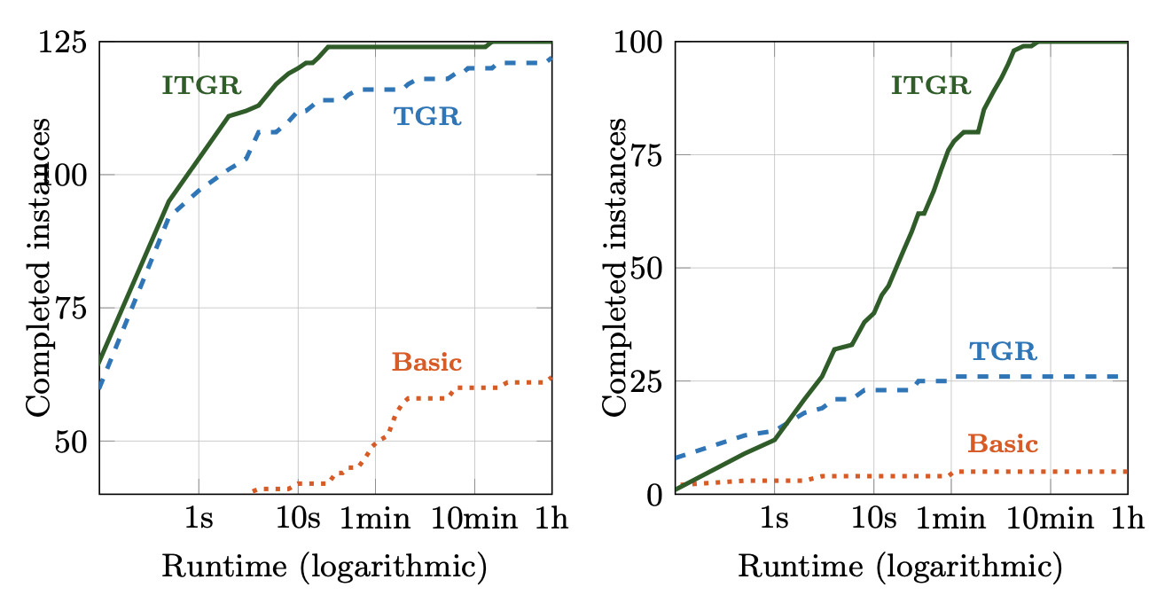
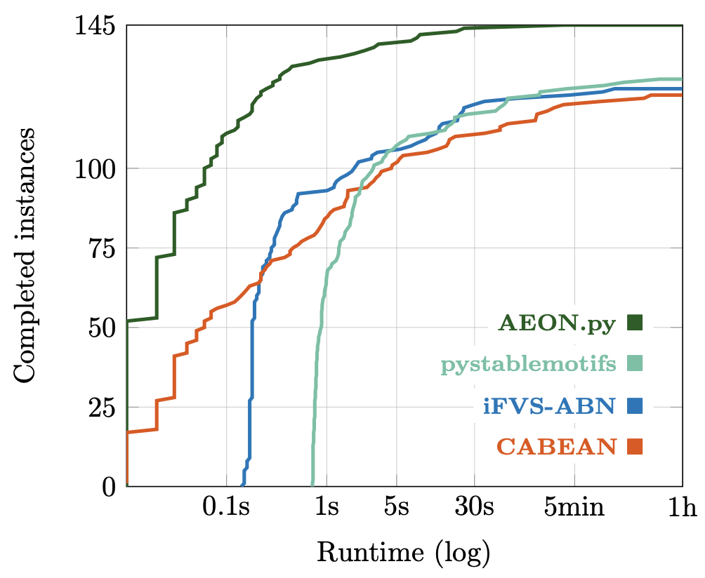
Are the colours actually useful?
Extrapolating from 1024 single-coloured samples over a smaller subset of models...
Anywhere from 100x to 5000x speed-up compared to a parameter scan.
Conclusions
- Symbolic algorithms can be surprising.
- Internal "parallelism" of the symbolic representation can often compute "more" faster than "less".
- Transition guided reduction: Filter states based on transitions that do not appear in (some) BSCCs.
- Interleaving smooths-out the edge cases.
Finding SCCs in many systems at once using symbolic algorithms
By Samuel Pastva


