Data-driven and Model-based Verification via Bayesian Identification and Reachability Analysis
ufff...
Experiment Setup
S
u(t)
\tilde{y}(t)
y(t)

e(t)
S \models \psi
???
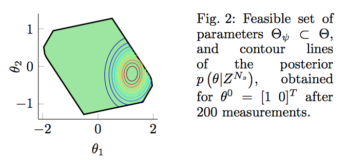
\text{Parameter set } \Theta
\text{Parametrised model } M(\theta) \mid \theta \in \Theta
\text{Family of parametrised models } \mathcal{G} = \{ M(\theta) \mid \theta \in \Theta \}
\text{Satisfaction function } f_{\psi}(\theta) = \textbf{P}(M(\theta)) \models \psi)
\text{mapping to } \{0,1\} \text{ or } [0,1]
\text{Sample size } N_s
\text{Sample } Z^{N_{s}} = \{ u(t), \tilde{y}(t) \}_{t=1}^{t=N_s}
\textbf{P} (S \models \psi | Z^{N_s}) = \int_{\Theta} f_{\psi}(\theta) p(\theta | Z^{N_s}) d\theta
\text{Bayesian confidence: }
p(\theta | Z^{N_s}) = \frac{p(Z^{N_s}|\theta)p(\theta)}{\int_{\Theta}p(Z^{N_s}|\theta)p(\theta)d\theta}
??
??
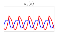
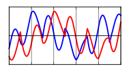
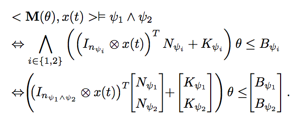
LTL over continuous signals
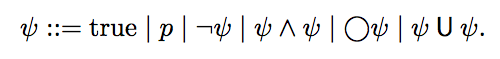
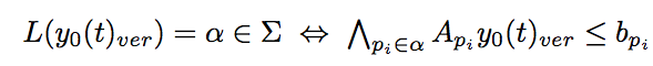
Atomic propositions: linear constraints in output space
Alphabet: Sets of atomic propositions (convex polytopes)
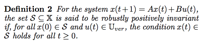
Models (LTI Systems)
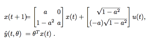
x(t+1) = A \cdot x(t) + B \cdot u(t)
Difference equations + output equations
y(t) = C(\theta) \cdot x(t) + D(\theta) \cdot u(t)
Only C and D are parametrised!
Non-linearly parametrised models can be approximated using orthonormal basis functions
How do we compute this?
How do we compute that?!
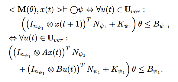
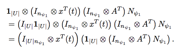
Several maths later...
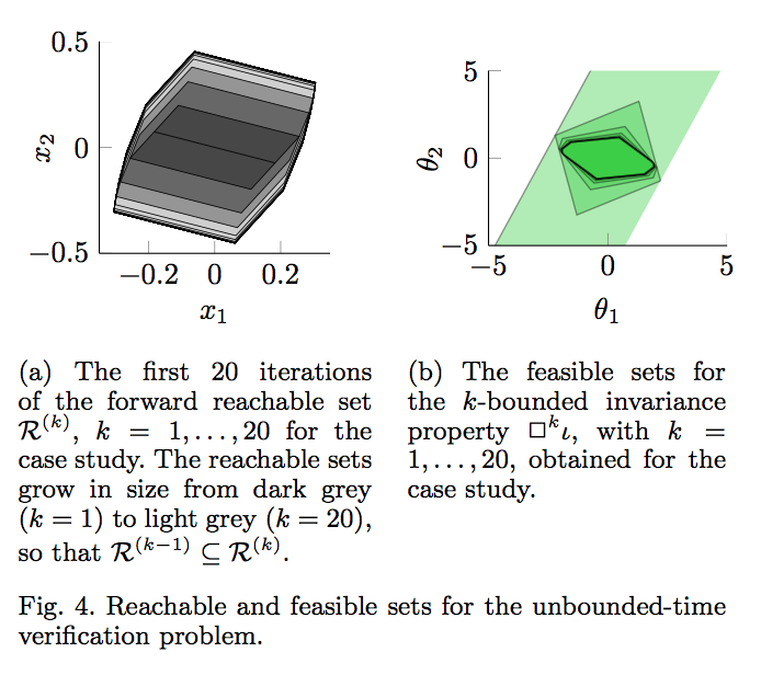
Bottom line: It is computable and the dimensionality depends on model and property
Bottom line: It is computable, assuming we know R, which can be approximated.
Bayesian Identification and Reachability Analysis
By Samuel Pastva


