Linear stability of fluid flows
What happens to analytical pertubations of fluid flows?
- Turbulence is a state of flow that needs to be created from something - an initial pertubation.
- It is completely impossible to perform fluid flow experiments without pertubations.
- A pipe flow has been kept stable for extremely large Re (> 10^6). Linear stability theory states that all straight pipe flows are stable...
- In the computer it is not difficult to create simulations free from pertubations or noise.
Linearization NS


Base flow + pertubation
Base eq:
Pertubation eq:
Linearize by deleting nonlinear underlined term

Linearization NS
Eliminate pressure by taking the divergence of the pert eq:


Eigenvalue problem
Consider separation of variables solutions of the form:


Leading to an eigenvalue problem:
Eigenvalue problem
Solutions with positive real eigenvalues are unstable. The pertubation will, obviously, grow in time
Likewise, solution with negative real eigenvalues will decay
With Linear Stability theory it is possible to say something absolute and concrete about whether or not a flow is likely to trigger turbulence!
Critical Reynolds numbers!
Consider the FDA case
Re = 3500
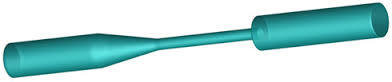
Two distinct regions
- Converging inlet section
- Impinging jet
Compute the flow field and compare with experiments
???
Extreme mesh sensitivity???
Enter LNS
Split the mesh into two regions
Compute the largest eigenvalue and eigenvector for each region separately
Enter LNS
Largest unstable eigenvalue/eigenvector pairs:
\lambda = -0.0382 + 0.0115 i
\lambda = 0.218+ 1.45 i
According to LNS flow should be stable in diverging part and unstable in jet - FDA reference data are turbulent in narrow pipe.
Offers an explanation for the extreme mesh sensitivity of Oasis
Further
-
Optimal growth of non-orthogonal pertubations
- Using adjoint NS
- Pulsatile flows - Floquet analysis
- Pseudo-spectra (Trefethen)
Optimal growth of pertubations
{u}' = \mathcal{M}(\tau)u'_0
\mathcal{M}(\tau) = \int_{t=0}^{t=\tau}\exp(\mathcal{L}(t)) dt
Operator reading: apply the linearized Navier–Stokes equations to an initial condition by
time-integration over interval
\tau
u'_0
Operator has the same eigenvectors as
Eigenvalues are related
\mathcal{M}
\mathcal{L}
\mu_j = \exp(\lambda_j \tau)
Non-orthogonal energy growth rate
\mathcal{M}^*
\frac{E(\tau)}{E(0)}=\frac{(u'_{\tau}, u'_{\tau})}{(u'_0, u'_0)}=\frac{(u'_0, \mathcal{M}^*\mathcal{M}u'_0)}{(u'_0, u'_0)}
where is adjoint operator of
\mathcal{M}
\mathcal{M}^*\mathcal{M}u'_0 = \frac{E(\tau)}{E(0)}u'_0
Study the eigensystem
to find the optimal (most dangerous) initial disturbance
deck
By Mikael Mortensen


