Amazon CoRo Kickoff
Oct 29 / Nov 18, 2024
Adam Wei
Agenda
- Motivation
- Cotraining & Problem Formulation
- Cotraining & Finetuning Insights
- New Algorithms for cotraining
- Future Work
Robot Data Diet

Big data
Big transfer gap
Small data
No transfer gap
Ego-Exo
robot teleop

Open-X
simulation
How can we obtain data for imitation learning?
Cotrain from different data sources
(ex. sim & real)
Motivation: Sim & Real Cotraining
Sim Infrastructure
Sim Data Generation

Motivation: Sim Data
- Simulated data is here to stay => we should understand how to use this data...
- Best practises for training from heterogeneous datasets is not well understood (even for real only)
Octo
DROID
Similar comments in OpenX, OpenVLA, etc...
Motivation: High-level Goals
... will make more concrete in a few slides
- Empirical sandbox results to inform cotraining practises
- Understand the qualities in sim data that affect performance
- Propose new algorithms for cotraining
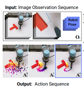
Problem Formulation
\mathcal{D}_{R}\sim p_{real}(O,A)
Robot Actions

O
A
\mathcal{D}_{S}\sim p_{sim}(O,A)


Robot Actions
A
O
- High quality data from the target distribution
- Expensive to collect
- Not the target distribution, but still informative data
- Scalable to collect
Problem Formulation
\mathcal{D}_{R}\sim p_{R}(O,A)
\mathcal{D}_S\sim p_{S}(O,A)
Cotraining: Use both datasets to train a model that maximizes some test objective
- Model: Diffusion Policy that learns \(p(A|O)\)
- Test objective: Empirical success rate on a planar pushing task
Notation
R, S => real and sim
\(|\mathcal D|\) = # demos in \(\mathcal D\)
\(\mathcal{L}=\mathbb{E}_{p_{O,A},k,\epsilon^k}[\lVert \epsilon^k - \epsilon(O_t, A^o_t + \epsilon^k, k) \rVert^2] \)
\(\mathcal{L}_{\mathcal{D}}=\mathbb{E}_{\mathcal{D},k,\epsilon^k}[\lVert \epsilon^k - \epsilon(O_t, A^o_t + \epsilon^k, k) \rVert^2] \approx \mathcal L \)
\(\mathcal D^\alpha\) Dataset mixture
- Sample from \(\mathcal D_R\) w.p. \(\alpha\)
- Sample from \(\mathcal D_S\) w.p, \(1-\alpha\)
Diffusion Policy Overview
Goal:
- Given data from an expert policy: \(p(A|O)\)
- Learn to sample from \(p(A|O)\)
Diffusion Policy:
- Learn a denoiser for \(p(A|O)\) and sample with diffusion
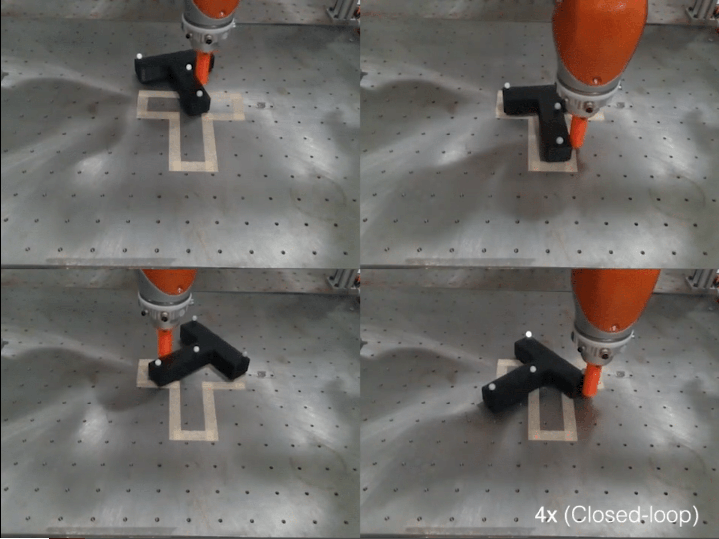
Task: Planar Pushing
- Simple problem, but encapsulates core challenges in contact-rich manipulation (hybrid system, control from pixels, etc)
- Allows for clean and controlled experiment design
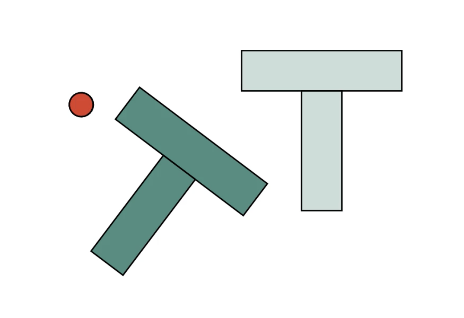
Goal: Manipulate object to target pose
Limitations
- The hope is that insights from planar pushing can generalize to other tasks and settings
Research Questions
- For vanilla cotraining: how do \(|\mathcal D_R|\), \(|\mathcal D_S|\), and \(\alpha\) affect the policy's success rate?
- How do distribution shifts affect cotraining?
- Propose new algorithms for cotraining
- Adversarial formulation
- Classifier-free guidance
Informs the qualities we want in sim

Vanilla Cotraining
\mathcal L_{\mathcal D^\alpha} = \alpha \textcolor{red}{\mathcal L_{\mathcal D_R}} + (1-\alpha) \textcolor{blue}{\mathcal L_{\mathcal D_S}}
(Tower property of expectations)
Vanilla Cotraining:
- Choose \(\alpha \in [0,1]\)
- Train a diffusion policy that minimizes \(\mathcal L_{\mathcal D^\alpha}\)
\(\mathcal D^\alpha\) Dataset mixture
- Sample from \(\mathcal D_R\) w.p. \(\alpha\)
- Sample from \(\mathcal D_S\) w.p, \(1-\alpha\)
Experiments
For vanilla cotraining: how do \(|\mathcal D_R|\), \(|\mathcal D_S|\), and \(\alpha\) affect the policy's success rate?
- Distributionally robust optimization, Re-Mix, etc
- Theoretical bounds
- Empirical approach
Experiment Setup
\(|\mathcal D_R|\) = 10, 50, 150 demos
\(|\mathcal D_S|\) = 500, 2000 demos
\(\alpha = 0,\ \frac{|\mathcal{D}_{R}|}{|\mathcal{D}_{R}|+|\mathcal{D}_{S}|},\ 0.25,\ 0.5,\ 0.75,\ 1\)
Sweep the following parameters:
For vanilla cotraining: how do \(|\mathcal D_R|\), \(|\mathcal D_S|\), and \(\alpha\) affect the policy's success rate?
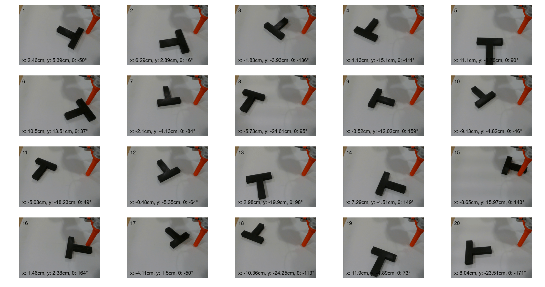
Experiment Setup
- Train for ~2 days on a single Supercloud V100
- Evaluate performance on 20 trials from matched initial conditions
Results
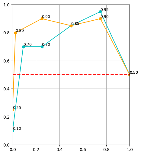
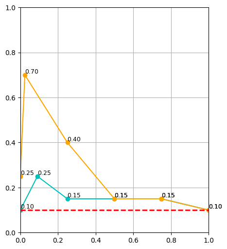

\(|\mathcal D_R| = 10\)
\(|\mathcal D_R| = 50\)
\(|\mathcal D_R| = 150\)
cyan: \(|\mathcal D_S| = 500\) orange: \(|\mathcal D_S| = 2000\) red: real only
Highlights
10 real demos
2000 sim demos
50 real demos
500 sim demos
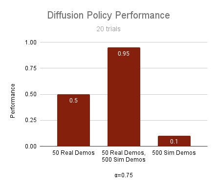
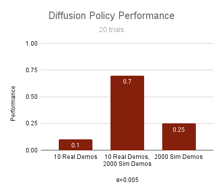
- Cotraining can drastically improve performance
Takeaways: \(\alpha\)
- Policy's are sensitive to \(\alpha\), especially when \(|\mathcal D_R|\) is small
- Smaller \(|\mathcal D_R|\) → smaller \(\alpha\)
- Larger \(|\mathcal D_R|\) → larger \(\alpha\)
- If \(|\mathcal D_R|\) is sufficiently large, sim data will not help. It also isn't detrimental.
Takeaways: \(|\mathcal D_R|\), \(|\mathcal D_S|\)
- Cotraining can improve policy performance at all data scales
- Scaling \(|\mathcal D_S|\) improves performance. This effect is drastically more pronouced for small \(|\mathcal D_R|\)
- Scaling \(|\mathcal D_S|\) reduces sensitivity of \(\alpha\)
Initial experiments suggest that scaling up sim is a good idea!
... to be verified at larger scales with sim-sim experiments
Cotraining Theory
\mathrm{prob\ of\ error} \leq \mathrm{bound}(\alpha,|\mathcal D_R|, |\mathcal D_S|, \mathrm{dist}(\mathcal D_R,\mathcal D_S), ...)
\alpha^*(|\mathcal D_R|, |\mathcal D_S|) = \argmin_{\alpha\in[0,1]} \mathrm{bound}(\alpha, |\mathcal D_R|, |\mathcal D_S|, ...)

Cotraining Theory
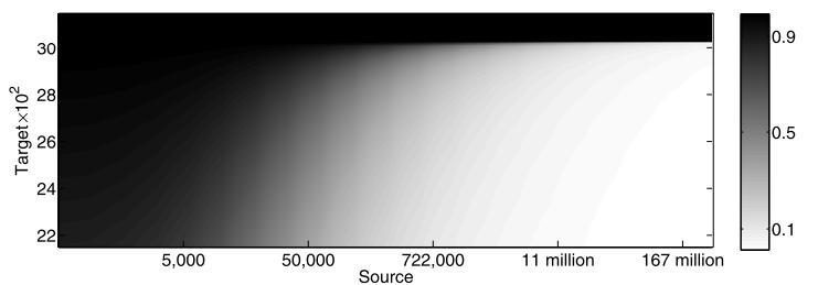
\(|\mathcal D_R|\)
\(|\mathcal D_S|\)
\alpha^*(|\mathcal D_R|, |\mathcal D_S|) = \argmin_{\alpha\in[0,1]} \mathrm{bound}(\alpha, |\mathcal D_R|, |\mathcal D_S|, ...)
Experiments match intuition and theoretical bounds
Finetuning Experiments
\(|\mathcal D_R|\) = 10, 50 demos
\(|\mathcal D_S|\) = 500, 2000 demos
Finetune a pretrained sim policy
- Cotrain a model on \(|\mathcal D_S|\) and \(|\mathcal D_R|\)
- Finetune with \(|\mathcal D_R|\)
Finetune a cotrained policy
- Pretrain a model on \(|\mathcal D_S|\)
- Finetune with \(|\mathcal D_R|\)
\(\implies\) 8 models, 20 trials each
Finetuning Results
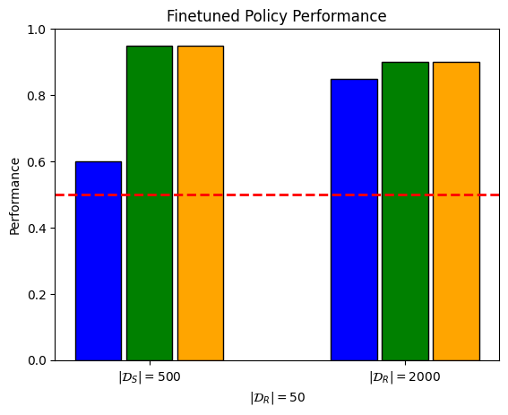
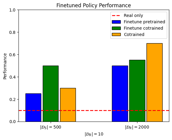
Takeaways
- Scaling \(|\mathcal D_S|\) improves performance for all algorithms
- Finetuning cotrained models > finetuning sim-only model
- In the single-task setting: finetuning does not appear to improve performance
Research Questions
- For vanilla cotraining: how do \(|\mathcal D_R|\), \(|\mathcal D_S|\), and \(\alpha\) affect the policy's success rate?
- How do distribution shifts affect cotraining?
-
New algorithms for cotraining
- Adversarial formulation
- Classifier-free guidance
Informs the qualities we want in sim
Distribution Shifts
Setting up a simulator for data generation is non-trivial
- camera calibration, colors, assets, physics, tuning, data filtering, task-specifications, etc
+ Actions
What qualities matter in the simulated data?
Distribution Shifts

Distribution Shifts
Visual Shifts
- Domain randomization
- Color shift
Physics Shifts
- Center of mass shift
Task Shifts
- Goal Shift
- Object shift


Original
Color Shift
Goal Shift
Object Shift
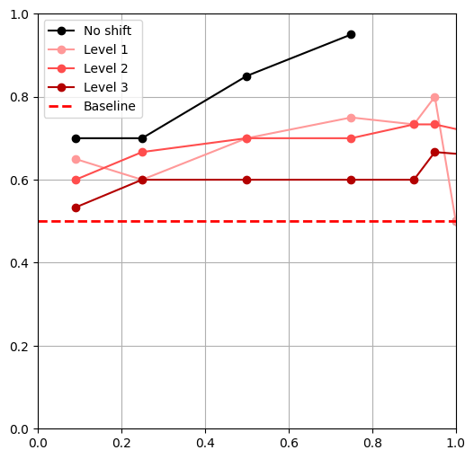
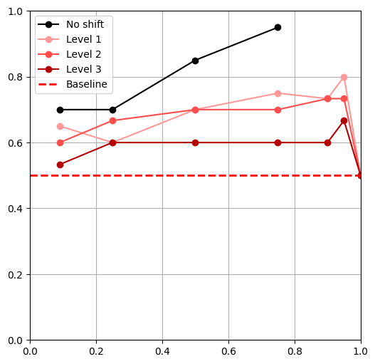
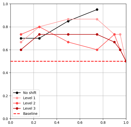
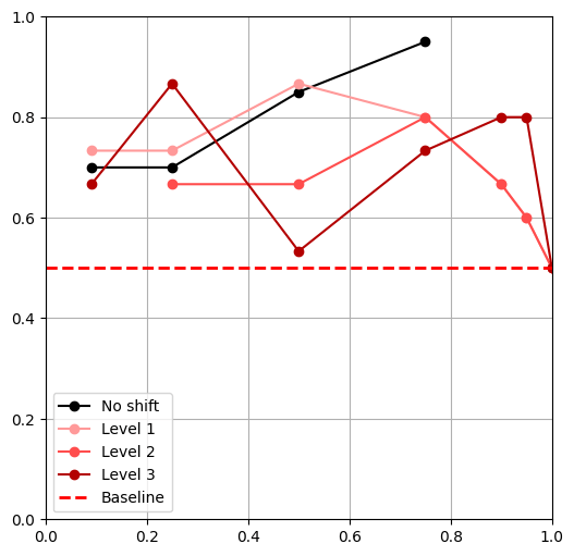
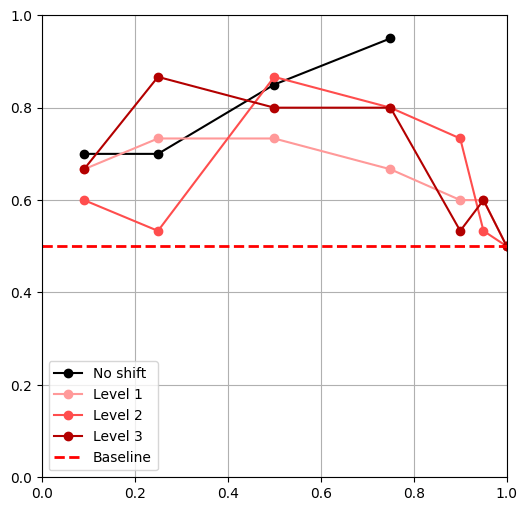
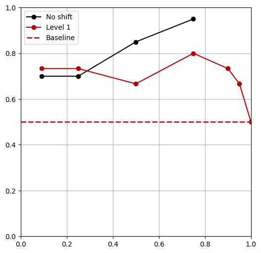
Distribution Shifts
Experimental Setup
- Tested 3 levels of shift for each shift**
- \(|\mathcal D_R|\) = 50, \(|\mathcal D_S|\) = 500,
- \(\alpha = 0,\ \frac{|\mathcal{D}_{R}|}{|\mathcal{D}_{R}|+|\mathcal{D}_{S}|},\ 0.25,\ 0.5,\ 0.75,\ 0.9,\ 0.95,\ 1\)
** Except object shift
Distribution Shifts
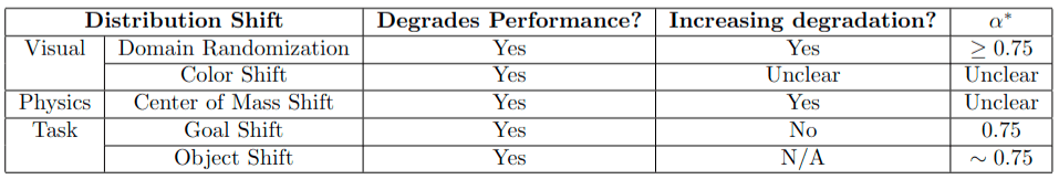
- All policies outperform the 'real only' baseline
Research question: Can we develop cotraining algorithms that mitigate the effects of distributions shifts?
Visual Shifts
Domain Randomization
Color Shift
Physics Shifts
Center of Mass Shift

Task Shifts
Goal Shift
Object Shift
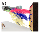
How does cotraining help?
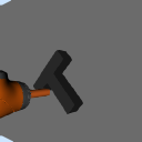
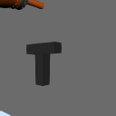
Sim Demos
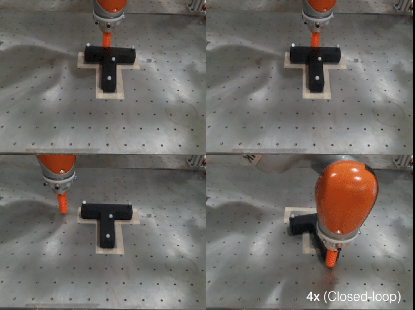
Real Rollout
Cotrained Policies
Cotrained policies exhibit similar characteristics to the real-world expert regardless of the mixing ratio
Real Data
- Aligns orientation, then translation sequentially
- Sliding contacts
- Leverage "nook" of T
Sim Data
- Aligns orientation and translation simultaneously
- Sticking contacts
- Pushes on the sides of T
How does cotraining improve performance?
Hypothesis
- Cotrained policies can identify the sim vs real: sim data helps by learning better representations and filling in gaps in real data
- Sim data prevents overfitting and acts as a regularizor
- Sim data provides more information about high probability unconditional actions \(p_A(a)\)
Probably some combination of the above.
Hypothesis 1: Binary classification
Cotrained policies can identify the sim vs real: sim data improves representation learning and fills in gaps in real data
| Policy | Observation embeddings acc. | Final activation acc. |
|---|---|---|
| 50/500, alpha = 0.75 | 100% | 74.2% |
| 50/2000, alpha = 0.75 | 100% | 89% |
| 10/2000, alpha = 0.75 | 100% | 93% |
| 10/2000, alpha = 5e-3 | 100% | 94% |
| 10/500, alpha = 0.02 | 100% | 88% |
Only a small amount of real data is needed to separate the embeddings and activations
Hypothesis 1: tSNE
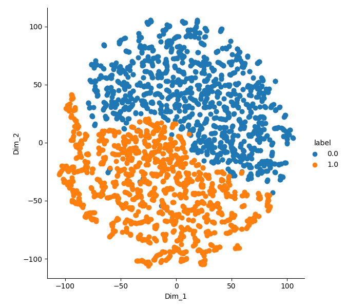
- t-SNE visualization of the observation embeddings
Hypothesis 1: kNN on actions
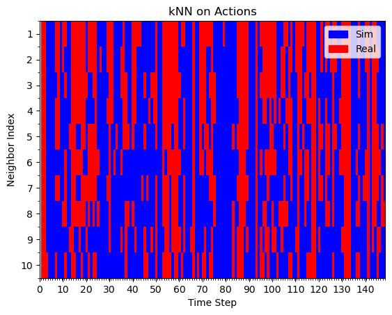

Real Rollout
Sim Rollout
Mostly red with blue interleaved
Mostly blue
Assumption: if kNN are real/sim, this behavior was learned from real/sim
Similar results for kNN on embeddings
Hypothesis 2
Sim data prevents overfitting and acts as a regularizor
\begin{aligned}
\mathcal{L_{train}}=\textcolor{red}{\mathcal{L}_{objective}} + \lambda\textcolor{blue}{\mathcal{L}_{regularizer}}
\end{aligned}
\mathcal L_{\mathcal D^\alpha} = \alpha \textcolor{red}{\mathcal L_{\mathcal D_R}} + (1-\alpha) \textcolor{blue}{\mathcal L_{\mathcal D_S}}
When \(|\mathcal D_R|\) is small, \(\mathcal L_{\mathcal D_R}\not\approx\mathcal L\).
\(\mathcal D_S\) helps regularize and prevent overfitting
Hypothesis 3
Sim data provides more information about \(p_A(a)\)
- i.e. improves the cotrained policies prior on "likely actions"
Can we test/leverage this hypothesis with classifier-free guidance?
... more on this later if time allows
Hypothesis
Research Questions
- How can we test these hypothesis?
- Can the underlying principles of cotraining help inform novel cotraining algorithms?
Hypothesis
Hypothesis
- Cotrained policies can identify the sim vs real: sim data helps by learning better representations and filling in gaps in real data
- Sim data prevents overfitting and acts as a regularizor
- Sim data provides more information about high probability actions \(p_A(a)\)
Example ideas:
- Hypothesis 1 \(\implies\) adversarial formulations for cotraining, digitial twins, representation learning, etc
- Hypothesis 3 \(\implies\) classifier-free guidance, etc
Research Questions
- For vanilla cotraining: how do \(|\mathcal D_R|\), \(|\mathcal D_S|\), and \(\alpha\) affect the policy's success rate?
- How do distribution shifts affect cotraining?
- Propose new algorithms for cotraining
- Adversarial formulation
- Classifier-free guidance
Sim2Real Gap
Thought experiment: what if sim and real were nearly indistinguishable?
- Less sensitive to \(\alpha\)
- Each sim data point better approximates the true denoising objective
- Improved cotraining bounds
Sim2Real Gap
Fact: cotrained models can distinguish sim & real
Thought experiment: what if sim and real were nearly indistinguishable?

Sim2Real Gap
\mathrm{prob\ of\ error} \leq \mathrm{bound}(\alpha,|\mathcal D_R|, |\mathcal D_S|, \mathrm{dist}(\mathcal D_R,\mathcal D_S), ...)
\(\mathrm{dist}(\mathcal D_R,\mathcal D_S)\) small \(\implies p^{real}_{(O,A)} \approx p^{sim}_{(O,A)} \implies p^{real}_O \approx p^{sim}_O\)
'visual sim2real gap'
Sim2Real Gap
Current approaches to sim2real: make sim and real visually indistinguishable
- Gaussian splatting, blender renderings, real2sim, etc
\(p^{R}_O \approx p^{S}_O\)
Do we really need this?
\(p^{R}_O \approx p^{S}_O\)
Sim2Real Gap
\(a^k\)
\(\hat \epsilon^k\)
\(o \sim p_O\)
\(o^{emb} = f_\psi(o)\)
\(p^{R}_O \approx p^{S}_O\)
\(p^{R}_{emb} \approx p^{S}_{emb}\)
\(\implies\)
Weaker requirement
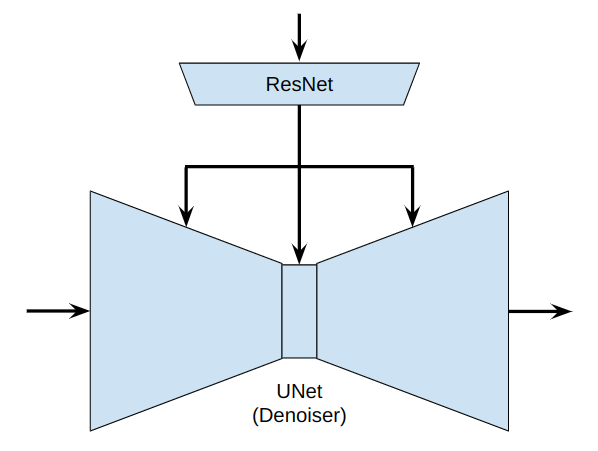
Adversarial Objective
\(\epsilon_\theta\)
\(f_\psi\)
\(d_\phi\)
\(\hat{\mathbb P}(f_\psi(o)\ \mathrm{is\ sim})\)
\(\epsilon^k\)
\(a^k\)
o
\min_{\theta, \psi} \mathcal L_{\mathcal D^\alpha}(\theta, \psi) + \lambda \max_\phi \mathbb E_{p^S_O}[\log d_\phi (f_\psi(o))] + \mathbb E_{p^R_O} [1-\log d_\phi (f_\psi(o))]
Adversarial Objective
\min_{\theta, \psi} \mathcal L_{\mathcal D^\alpha}(\theta, \psi) + \lambda \max_\phi \mathbb E_{p^S_O}[\log d_\phi (f_\psi(o))] + \mathbb E_{p^R_O} [1-\log d_\phi (f_\psi(o))]
Denoiser Loss
Negative BCE Loss
\(\iff\)
\min_{\theta, \psi} \mathcal L_{\mathcal D^\alpha}(\theta, \psi) + \lambda \cdot \mathrm{JS}(p^S_{emb}, p^R_{emb})
(Variational characterization of f-divergences)
Adversarial Objective
\min_{\theta, \psi} \mathcal L_{\mathcal D^\alpha}(\theta, \psi) + \lambda \cdot \mathrm{JS}(p^S_{emb}, p^R_{emb})
Common features (sim & real)
- End effector position
- Object keypoints
- Contact events
Distinguishable features*
- Shadows, colors, textures, etc
Relavent for control...
- Adversarial objective discourages the embeddings from encoding distinguishable features*
* also known as protected variables in AI fairness literature
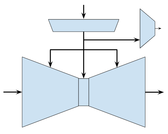
Adversarial Objective
\(\epsilon_\theta\)
\(f_\psi\)
\(d_\phi\)
\(\hat{\mathbb P}(f_\psi(o)\ \mathrm{is\ sim})\)
\(\epsilon^k\)
\(a^k\)
o
\min_{\theta, \psi} \mathcal L_{\mathcal D^\alpha}(\theta, \psi) + \lambda \max_\phi \mathbb E_{p^S_O}[\log d_\phi (f_\psi(o))] + \mathbb E_{p^R_O} [1-\log d_\phi (f_\psi(o))]
Adversarial Objective
\min_{\theta, \psi} \mathcal L_{\mathcal D^\alpha}(\theta, \psi) + \lambda \max_\phi \mathbb E_{p^S_O}[\log d_\phi (f_\psi(o))] + \mathbb E_{p^R_O} [1-\log d_\phi (f_\psi(o))]
Denoiser Loss
Negative BCE Loss
\(\iff\)
\min_{\theta, \psi} \mathcal L_{\mathcal D^\alpha}(\theta, \psi) + \lambda \cdot \mathrm{JS}(p^S_{emb}, p^R_{emb})
(Variational characterization of f-divergences)
Adversarial Objective
\min_{\theta, \psi} \mathcal L_{\mathcal D^\alpha}(\theta, \psi) + \lambda \cdot \mathrm{JS}(p^S_{emb}, p^R_{emb})
Hypothesis:
- Less sensitive to \(\alpha\)
- Less sensitive to visual distribution shifts
- Improved performance for \(|\mathcal D_R|\) = 10
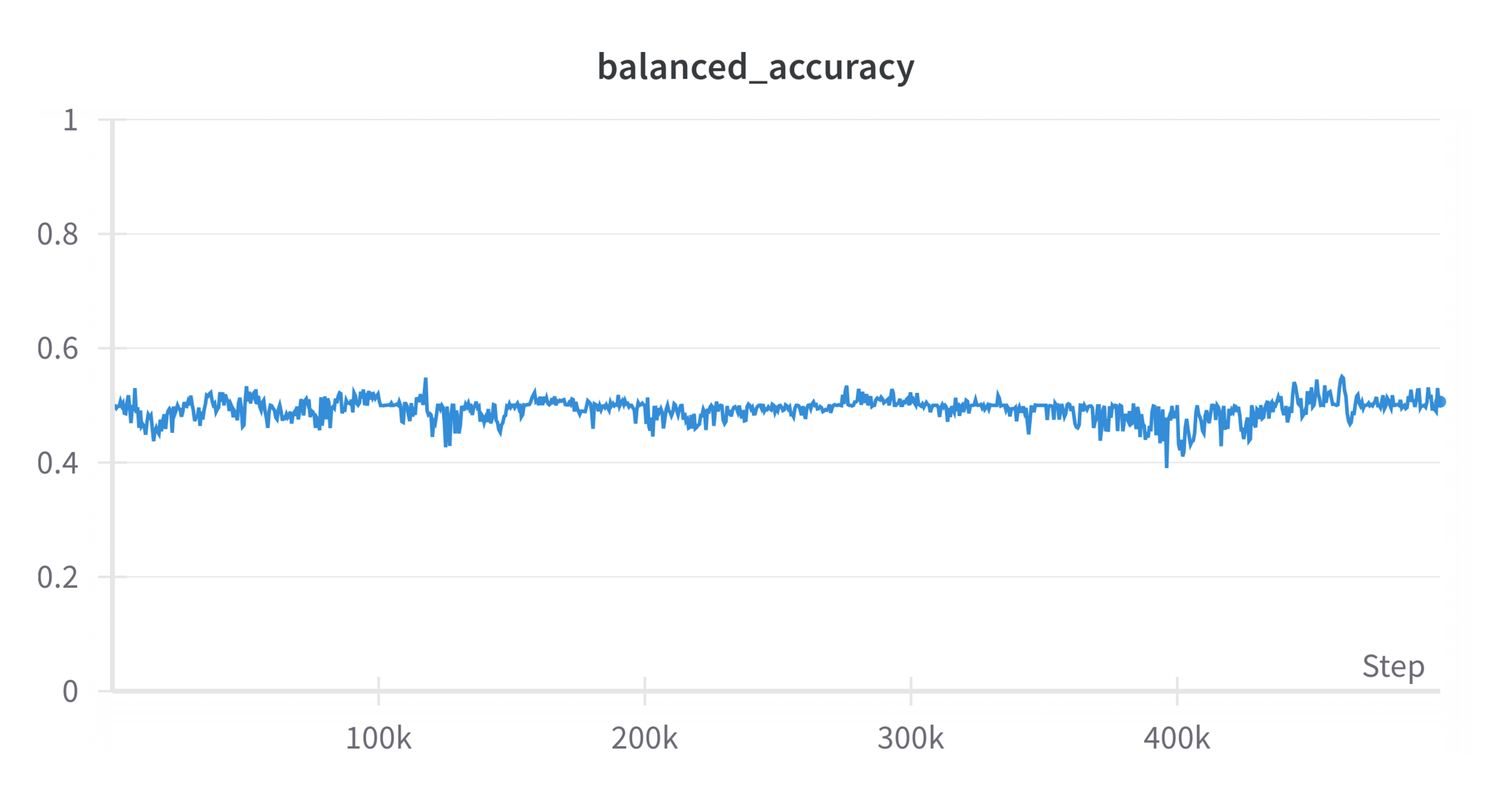
Initial Results
\(|\mathcal D_R| = 50\), \(|\mathcal D_S| = 500\), \(\lambda = 1\), \(\alpha = 0.5\)
Performance: 9/10 trials
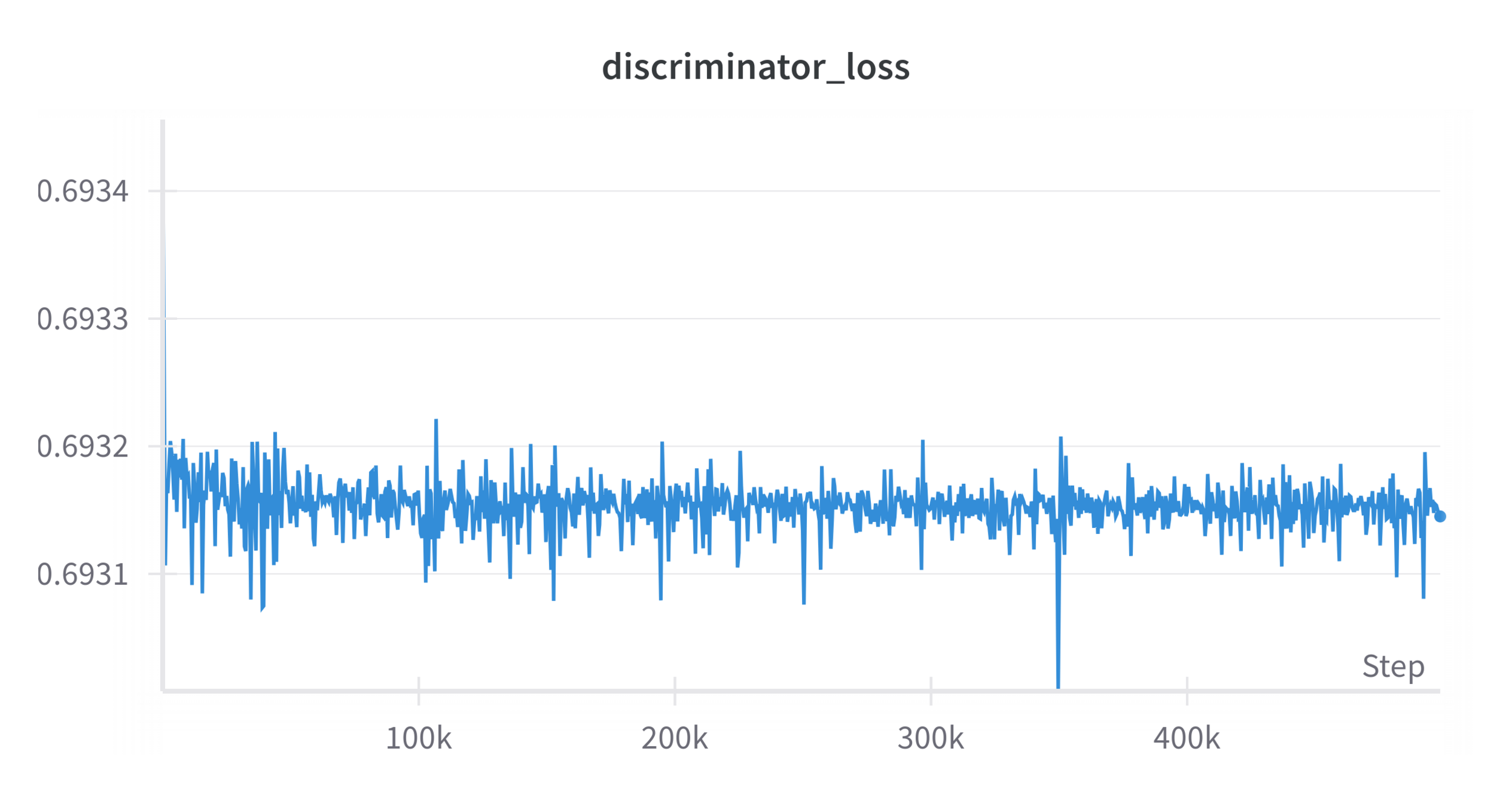
~log(2)
~50%
Problems...
-
A well-trained discriminator can still distinguish sim & real
- This is an issue with the GAN training process (during training, the discriminator cannot be fully trained)
- Image GAN models suffer similar problems
Potential solution?
- Place the discriminator at the final activation?
- Wasserstein GANs (WGANs)
\min_{\theta, \psi} \mathcal L_{\mathcal D^\alpha}(\theta, \psi) + \lambda \cdot \mathrm{W}(p^S_{emb}, p^R_{emb})
Two Philosophies For Cotraining
1. Minimize sim2real gap
- Pros: better bounds, more performance from each data point
- Cons: Hard to match sim and real, adversarial formulation assumes protected variables are not relevant for control
2. Embrace the sim2real gap
- Pros: policy can identify and adapt strongly to its target domain at runtime, do not need to match sim and real
- Cons: Doesn't enable "superhuman" performance, potentially less data efficient
Hypothesis 3
Sim data provides more information about \(p_A(a)\)
- Sim data provides a strong prior on "likely actions" =>improves the performance of cotrained policies
We can explicitly leverage this prior using classifier free guidance
\tilde\epsilon_\theta(O, A^k,k) = (1+\omega)\epsilon_\theta(O, A^k,k) - \omega\epsilon_\theta(\emptyset, A^k,k)
Conditional Score Estimate
Unconditional Score Estimate
Helps guide the diffusion process
\mathrm{better\ est. of\ } p_A \implies \mathrm{better\ } \epsilon_\theta(\emptyset, A^k,k)
Classifier-Free Guidance
\begin{aligned}
\tilde\epsilon_\theta(O, A^k,k) &= (1+\omega)\epsilon_\theta(O, A^k,k) - \omega\epsilon_\theta(\emptyset, A^k,k)\\
&=\epsilon_\theta(O, A^k,k) + \omega(\epsilon_\theta(O, A^k,k) - \epsilon_\theta(\emptyset, A^k,k))
\end{aligned}
Conditional Score Estimate
- Term 2 guides conditional sampling by separating the conditional and unconditional action distributions
- In image domain, this results in higher quality conditional generation

Difference in conditional and unconditional scores
Classifier-Free Guidance
\begin{aligned}
\tilde\epsilon_\theta(O, A^k,k) &= (1+\omega)\epsilon_\theta(O, A^k,k) - \omega\epsilon_\theta(\emptyset, A^k,k)\\
&=\epsilon_\theta(O, A^k,k) + \omega(\epsilon_\theta(O, A^k,k) - \epsilon_\theta(\emptyset, A^k,k))
\end{aligned}
- Due to the difference term, classifier-free guidance embraces the differences between \(p^R_{(A|O)}\) and \(p_A\)
- Note that \(p_A\) can be provided scalably by sim and also does not require rendering observations!
Future Work
- Evaluating scaling laws (sim-sim experiments)
- Adversarial and classifier-free guidance formulations
Immediate next steps:
Guiding Questions:
- What are the underlying principles and mechanisms of cotraining? How can we test them?
- Can we leverage these principles for algorithm design?
- Should cotraining minimize or embrace the sim2real gap?
- How can we cotrain from non-robot data (ex. video, text, etc)?
Amazon Kickoff
By Adam Wei


