Truth in the Age of Deep Learning
Building a model-selection criterion which survives replication
Alexandre René
rene@netsci.rwth-aachen.de
D-IEP semiar • 6 Nov 2025 • Amsterdam


Follow along

https://alcrene.github.io/emd-paper
Paper (HTML)

These slides
https://slides.com/alexrene/
truth-in-the-age-of-dl

Paper (PDF)
https://doi.org/10.1038/s41467-025-64658-7
PyPI package
https://pypi.org/project/emdcmp

Executable capsule
https://codeocean.com/capsule/0868474/tree/v1

Usual scientific workflow
Anecdotal
observations
What we want in a Selection Criterion
Usual scientific workflow
Conceive theory
Conceive experiment
Accumulate data
Compare
Make prediction
New experiment?
Assumptions
Symmetry
Conservation
Exchangeability
Anecdotal
observations
Validate/falsify
- High-level goal is induction
- Objective is predictive accuracy
- No model is perfect
- The amount of data is undetermined
What we want in a Selection Criterion

Prinz et al., Nat Neurosci (2004)
René, Pyloric simulator, PyPI (2025)
C_a \frac{dV}{dt} = \;\;\sum_{\mathclap{\text{ion channels}}}\; \bar{g}_i m_i[V]^p h_i[V] (V - E_i)
\begin{aligned}
\mathcal{B}_{\mathrm{RJ}}(λ; T) &= \frac{2 c k_B T}{λ^4} \\
\mathcal{B}_\mathrm{P}(λ; T) &= \frac{2 h c^2}{λ^5} \frac{1}{\exp\left( \frac{hc}{λ k_B T} \right) - 1}
\end{aligned}
Two model examples
Radiance of a Black Body
Neurons of the Crustacean Pyloric Circuit
Fitting parameters
→ Distinct local solutions
- Two model candidates
- Models ↔
Different equations
Different parameters
- Two model candidates
- Models ↔
Same equations
Different parameters
Rayleigh-Jeans
Planck
Standard statistical criteria
EMD criterion

Prinz et al., Nat Neurosci (2004)
René, Pyloric simulator, PyPI (2025)
C_a \frac{dV}{dt} = \;\;\sum_{\mathclap{\text{ion channels}}}\; \bar{g}_i m_i[V]^p h_i[V] (V - E_i)
\begin{aligned}
\mathcal{B}_{\mathrm{RJ}}(λ; T) &= \frac{2 c k_B T}{λ^4} \\
\mathcal{B}_\mathrm{P}(λ; T) &= \frac{2 h c^2}{λ^5} \frac{1}{\exp\left( \frac{hc}{λ k_B T} \right) - 1}
\end{aligned}
Two model examples
Radiance of a Black Body
Neurons of the Crustacean Pyloric Circuit
- Two model candidates
- Models ↔
Different equations
Different parameters
- Two model candidates
- Models ↔
Same equations
Different parameters
Rayleigh-Jeans
Planck
\left\{\begin{aligned}
&\mathcal{M}_A \\
&\;\;\;\vdots \\
&\mathcal{M}_Z
\end{aligned}\right\}
\left\{\begin{aligned}
&\mathcal{M}_C \\
&\mathcal{M}_E \\
&\mathcal{M}_P
\end{aligned}\right\}
Goal
selection
criterion
- Only reject if enough evidence
⤷No forced choiced
We will use risk: \(\mathbb{E}_{\mathcal{M}_{\mathrm{true}}}[Q]\) to rank models
Some loss
\(θ_A\) subsumed into \(\mathcal{M}_A\)

The problem with Forced Choice
Data
Empirical Risk
Not all comparisons should be conclusive
Result is not consistent across replications
Intuition: More predictive accuracy ⇒ More reliable comparison
Why? If we know a source of variable, we can:
- account for it in the model
- control for it in the experiment
EMD assumption: Model discrepancies are due to unknown variability
Unknown sources of variability may change across experiments

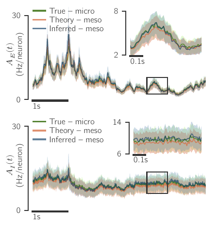
- Empirical risk accounts for predictive performance and non-stationary replications (aka generalization)
(“consistency”) - But still a forced choice: no notion of uncertainty
- We are going to construct a criterion which bootstraps epistemic uncertainty from prediction discrepancies:
Empirical Modelling Discrepancy (EMD)
Ranking models based on empirical risk
\(R\): Risk
(lower is better)
Are these differences in risk all meaningful?
Data
Pointwise loss
(Empirical) risk
\((x_i, y_i) \sim \mathcal{D}_{\mathrm{true}} \)
\(Q(x_i, y_i \mid \mathcal{M}_A) \to \mathbb{R}\)
\(\mathbb{E}\bigl[Q(x_i, y_i \mid \mathcal{M}_A) \bigr] \approx \frac{1}{L} \;\sum\limits_{\mathclap{\qquad(x_i, y_i) \sim \mathcal{D}_{\mathrm{true}}}}\;\; Q(x_i, y_i \mid \mathcal{M}_A) \)
NB: \(θ\) subsumed into \(\mathcal{M}_a\)
We assume to have
- \(\bigl\{\mathcal{M}_A, \mathcal{M}_B, \dotsc \bigr\}\)
each defining \(p(x_i, y_i \mid \mathcal{M}_a) \) - \(Q: \mathcal{X} \times \mathcal{Y} \to \mathbb{R} \)
- ability to sample \(\mathcal{M}_{\mathrm{true}}\)
How do we measure this?
And turn it into this?
Discrepancy
Model ↔ Quantile Function

For purposes of calculating risk, we can reduce any model to \(q(Φ)\) without loss of information
\begin{aligned}
R_A &:= \mathbb{E}_{\mathcal{M}_\mathrm{true}}\bigl[Q(x_i, y_i \mid \mathcal{M}_A) \bigr] \\
&\;= \int_{\mathcal{X}\times\mathcal{Y}}
\hspace{-18mu} dxdy\, p(x,y \mid \mathcal{M}_{\mathrm{true}}) \; Q(x, y \mid \mathcal{M}_A) \\
&\;= \int_{-\infty}^\infty \hspace{-12mu} dq
\int_{\substack{\\\!\!\!\!\!\mathcal{X}\times\mathcal{Y}\\\!\!\!Q(x,y)=q}}
\hspace{-32mu} dxdy\,p(x,y \mid \mathcal{M}_{\mathrm{true}}) \; Q(x, y \mid \mathcal{M}_A) \\
&\;= \int_{-\infty}^\infty \hspace{-6mu} dq \;q\; p(q \mid \mathcal{M}_\mathrm{true}, \mathcal{M}_A) \\
&\;= \int_{-\infty}^\infty \hspace{-6mu} dq \;q(Φ \mid \mathcal{M}_\mathrm{true}, \mathcal{M}_A) \frac{d}{dq} Φ \\
R_A &\;= \int_{0}^{1} q(Φ\mid \mathcal{M}_\mathrm{true}, \mathcal{M}_A) dΦ
\end{aligned}
\begin{aligned}
\vphantom{Φ(q \mid \mathcal{M}_{\mathrm{true}}, \mathcal{M}_A)}
Φ(q \mid \dots)
&= \int_{\substack{\\\!\!\!\!\!\mathcal{X}\times\mathcal{Y}\\\!\!\!Q(x,y){\color{blue} \bm{\leq}} q}}
\hspace{-32mu} dxdy\; Q(x, y \mid \mathcal{M}_A) p(x,y \mid \mathcal{M}_{\mathrm{true}}) \\[5ex]
&\approx \frac{1}{\lvert \mathcal{D} \rvert} \sum_{\mathcal{D}} \bigl[ Q(x,y) \leq q \bigr]
\end{aligned}
R_A \;= \int_{0}^{1} q(Φ \mid \mathcal{M}_\mathrm{true}, \mathcal{M}_A) dΦ \quad {\color{grey} \approx \frac{1}{\lvert \mathcal{D} \rvert} \sum_{(x,y)\in\mathcal{D}} Q(x,y \mid \mathcal{M}_A)}
Model ↔ Quantile Function
For purposes of calculating risk, we can reduce any model to \(q(Φ)\) without loss of information
EMD assumption (reframed): Candidate models represent that part of the experiment which we understand and control across replications

We can estimate \(R_A\) in two different ways:
\tilde{R}_A = \int_{\mathcal{X}\times\mathcal{Y}}
\hspace{-18mu} dxdy\; Q(x, y \mid {\color{blue} \mathcal{M}_A}) p(x,y \mid {\color{blue} \mathcal{M}_A}) \\
R_A^* = \int_{\mathcal{X}\times\mathcal{Y}}
\hspace{-18mu} dxdy\; Q(x, y \mid {\color{blue} \mathcal{M}_A}) p(x,y \mid {\color{blue} \mathcal{M}_{\mathrm{true}}}) \\
Mixed \(q_A^*\)
Synth \(\tilde{q}_A\)
Repeat for each \(\mathcal{M}\)
Stochastic Processes on Quantile Functions
Desiderata
Any process \(\mathcal{Q}\) should be
- monotone
- integrable
- non-accumulating
\mathbb{E}\bigl[ \lvert q(Φ + ΔΦ) - q(Φ) \rvert \bigr] \lesssim C \, ΔΦ
There is no way to coax a Wiener process to yield what we need

Variance must not depend on \(Φ\), only on \(δ^{\mathrm{EMD}}(Φ)\)
- \(\hat{q}\) should be “centered” on \(q^*\)
- The “variability” of \(\hat{q}\) should be proportional to \(\color{#FF7b00} δ^{\mathrm{EMD}}\)
\begin{aligned}
&\tilde{q}(Φ+ΔΦ) \\
&\quad= \tilde{q}(Φ) + \mathcal{N}\bigl[q^*(Φ+ΔΦ) - q^*(Φ), c(δ^{\mathrm{EMD}})^2\bigr]
\end{aligned}
Hierarchical Beta Process on Quantile Functions
Instead of accumulating increments left-to-right, we successively refine the interval
We draw increment pairs, under the constraint
\(Δq_{ΔΦ}(Φ) \stackrel{!}{=} Δq_{ΔΦ/2}(Φ) + Δq_{ΔΦ/2}(Φ+ΔΦ/2)\)
\Rightarrow
We need a compositional distribution
Mateu-Figueras et al., Distributions on the Simplex Revisited, 2021
The simplest 2-D compositional distributon is the beta distribution
\begin{aligned}
&\tilde{q}(Φ+ΔΦ) \\
&\quad= \tilde{q}(Φ) + \mathcal{N}\bigl[q^*(Φ+ΔΦ) - q^*(Φ), c(δ^{\mathrm{EMD}})^2\bigr]
\end{aligned}

Φ
ΔΦ = 2^{-1}
Φ
ΔΦ = 2^{-2}
Φ
ΔΦ = 2^{-3}
q
Φ
q
Φ
ΔΦ = 2^0
Hierarchical Beta Process on Quantile Functions
We draw increment pairs, under the constraint
\(Δq_{ΔΦ}(Φ) \stackrel{!}{=} Δq_{ΔΦ/2}(Φ) + Δq_{ΔΦ/2}(Φ+ΔΦ/2)\)
Φ
q
Φ
Beta
\begin{alignedat}{7}
x &\sim \mathop{\mathrm{Beta}} &&\Rightarrow\; & p(x) &\propto x^α (1 - x)^β &&\,,& \quad x &\in [0, 1] \\
\phantom{x_1, x_2}&\phantom{\sim \mathop{\mathrm{Beta}}} &&\phantom{\Rightarrow\;} & \phantom{p(x_1,x_2)} &\phantom{\propto x_1^α\;\; x_2^β} &&\phantom{\,,}& \phantom{\quad x_1,x_2} &\phantom{\in [0, 1], \, x_1 + x_2 \stackrel{!}{=} 1}
\end{alignedat}
Compositional form
Desiderata
- monotone
- integrable
- non-accumulating
\left.\begin{aligned}
\\[4ex]
\end{aligned}\right\}
By construction
- \(\hat{q}\) should be “centered” on \(q^*\)
\left.\begin{aligned}
\\[4ex]
\end{aligned}\right\}
Determine \(α\) and \(β\)
\begin{alignedat}{7}
\phantom{x} &\phantom{\sim \mathop{\mathrm{Beta}}} &&\phantom{\Rightarrow\;} & \phantom{p(x)} &\phantom{\propto x^α (1 - x)^β} &&\,\phantom{,}& \quad \phantom{x} &\phantom{\in [0, 1]} \\
x_1, x_2&\sim \mathop{\mathrm{Beta}} &&\Rightarrow\; & p(x_1,x_2) &\propto x_1^α\;\; x_2^β &&\,,& \quad x_1,x_2 &\in [0, 1], \, x_1 + x_2 \stackrel{!}{=} 1
\end{alignedat}
- The “variability” of \(\hat{q}\) should be proportional to \(\color{#FF7b00} δ^{\mathrm{EMD}}\)
Hierarchical Beta Process on Quantile Functions
We draw increment pairs, under the constraint
\(Δq_{ΔΦ}(Φ) \stackrel{!}{=} Δq_{ΔΦ/2}(Φ) + Δq_{ΔΦ/2}(Φ+ΔΦ/2)\)
Φ
q
Φ
Beta
\begin{alignedat}{7}
\phantom{x} &\phantom{\sim \mathop{\mathrm{Beta}}} &&\phantom{\Rightarrow\;} & \phantom{p(x)} &\phantom{\propto x^α (1 - x)^β} &&\,\phantom{,}& \quad \phantom{x} &\phantom{\in [0, 1]} \\
x_1, x_2&\sim \mathop{\mathrm{Beta}} &&\Rightarrow\; & p(x_1,x_2) &\propto x_1^α\;\; x_2^β &&\,,& \quad x_1,x_2 &\in [0, 1], \, x_1 + x_2 \stackrel{!}{=} 1
\end{alignedat}
- \(\hat{q}\) should be “centered” on \(q^*\)
- The “variability” of \(\hat{q}\) should be proportional to \(\color{#FF7b00} δ^{\mathrm{EMD}}\)
Because of the constraint, mean and variance are not natural statistics for compositional distributions
Mateu-Figueras et al., Distributions on the Simplex Revisited, 2021
Instead it is better to use the center and metric variance
\mathbb{E}_a[(x_1, x_2)] = \frac{1}{e^{ψ(α)} + e^{ψ(β)}} \bigl(e^{ψ(α)}, e^{ψ(β)}\bigr)
\mathop{\mathrm{Mvar}}[(x_1, x_2)] = \frac{1}{2} \bigl(ψ_1(α) + ψ_1(β)\bigr)
Two equations ⇒ Solve for \(α\) and \(β\)
\frac{e^{ψ(α)}}{e^{ψ(β)}} \stackrel{!}{=} \frac{Δq_{ΔΦ}^*(Φ)}{Δq_{ΔΦ}^*(Φ+ΔΦ)}
\mathop{\mathrm{Mvar}}[(x_1, x_2)] \stackrel{!}{=} c\,δ^\mathrm{EMD}
Hierarchical Beta Process on Quantile Functions
q
Φ
A Qualitatively Different Criterion


Dataset size
“Strength” of evidence
BIC
Bayes factor
MDL
AIC
elpd
- No
- Partially —
vol(posterior) - No
- No
- No
- No
- Yes —
vol(posterior) - No
- No
- No
- No
- Yes — ability to fit arb. data
- No
- No
- No
- Partially — unbiased est.
-
No
- No
- No
- No
-
Yes
-
No
- No
- No
- No
EMD
- High-level goal is induction
- Objective is predictive accuracy
- No model is perfect
- The amount of data is undetermined
- Considers generalization error
- Penalizes model complexity
- Allows for misspecified models
- Allows for non-stationary replications
- Bounded discriminability (as \(\lvert\mathcal{D}\rvert \to \infty\))
-
Yes
-
No
- No
- No
- No

Calibration: Putting units on the proportionality
\bm{ δ^\mathrm{EMD} }
\mathop{\mathrm{Mvar}}[(x_1, x_2)] \stackrel{!}{=} {\color{1692ad} c} \,δ^\mathrm{EMD}
- Converts discrepancy to metric variance
- Context-dependent: chosen by
simulating experimental variations
Procedure
- Use domain & problem knowledge to define “epistemic distributions” \(Ω\) over
- weak vs strong input
- data correlations
- temperature
- …
- Simulate 1000’s of model comparisons for each tested value of \(c\)
- Compare to the ground truth probabilities
- Select a \(c\) which systematically underestimates selection confidence
B^\mathrm{EMD}_{AB} := P(R_A < R_B \mid c)
Use the fact that \(B^\mathrm{EMD}_{AB}\) are true probabilities:
B^\mathrm{epis}
Calibration: Putting units on the proportionality
\bm{ δ^\mathrm{EMD} }
Procedure
- Use domain & problem knowledge to define “epistemic distributions” \(Ω\) over
- weak vs strong input
- data correlations
- temperature
- …
- Simulate 1000’s of model comparisons for each tested value of \(c\)
- Compare to the ground truth probabilities
- Select a \(c\) which systematically underestimates selection confidence
B^\mathrm{EMD}_{AB} := P(R_A < R_B \mid c)
Use the fact that \(B^\mathrm{EMD}_{AB}\) are true probabilities:
(white region)
B^\mathrm{epis}
(true)
(theory)
Summary – Ideas
Φ
R_A \;= \mathbb{E}_{\mathcal{M}_\mathrm{true}}\bigl[Q(x_i, y_i \mid \mathcal{M}_A) = \int_{0}^{1} dΦ(q \mid \mathcal{M}_\mathrm{true}, \mathcal{M}_A)
Summary – Procedure
Repeat for each \(\mathcal{M}\)
Calibration
Summary – Procedure
Repeat for each \(\mathcal{M}\)
Calibration
All of this can be automated
emdcmp on PyPI
from emdcmp import Bemd, make_empirical_risk, draw_R_samples

synth_ppfA = make_empirical_risk(lossA(modelA.generate(Lsynth)))
synth_ppfB = make_empirical_risk(lossB(modelB.generate(Lsynth)))
mixed_ppfA = make_empirical_risk(lossA(data))
mixed_ppfB = make_empirical_risk(lossB(data))

Bemd(mixed_ppfA, mixed_ppfB, synth_ppfA, synth_ppfB, c=c)
Thank You
Chair of Computational Network Science
(Prof. Michael Schaub)


netsci.rwth-aachen.de
Alexandre René
rene@netsci.rwth-aachen.de
www.arene.ca
HOOC Workshop takes place here
(cerca August 2026)
Extra slides
We can learn more, and more complex, models

Multiple LP candidates with similar responses
Prinz et al., Nat Neurosci (2004)
René, pyloric simulator, PyPI (2025)
C_a \frac{dV}{dt} = \;\;\sum_{\mathclap{\text{ion channels}}}\; \bar{g}_i m_i[V]^p h_i[V] (V - E_i)
8D Parameter sweep
… arguably too many models

t_k
t_{k-1}
t_{k-2}
…
\nabla_{\color{#3cb100} Θ}

René et al., Neural Comp (2020)
Back-propagation through time
What kind of robustness do we seek?
Variations
At a large scale, what kinds of variations do we want to account for?
- In-distribution data
- Out-of-distribution data
- Model parameters
High-level
Paradigm
How do we define/quantify these variations and the selection objective?
Specific
- Epistemic distribution (\(Ω\))
- Data-generating process (\(\mathcal{M}_{\mathrm{true}}\))
- Dataset (\(\mathcal{D}\))
- Parameters (\(θ\))
- Score function (\(R\))
- Evaluate score on…
Properties
Higher-level assessment.
These follow from the choice of paradigm.
Functional
- Considers generalization error
- Penalizes model complexity
- Allows for misspecified models
- Allows for non-stationary replications
- Bounded discriminability (as \(L \to \infty\))
Different criteria ↔ Different notions of robustness
Variations
Paradigm
Properties
- In-distribution data
- Out-of-distribution data
- Model parameters
- Epistemic distribution (\(Ω\))
- Data-generating process (\(\mathcal{M}_{\mathrm{true}}\))
- Dataset (\(\mathcal{D}\))
- Parameters (\(θ\))
- Score function (\(R\))
- Evaluate score on…
- Considers generalization error
- Penalizes model complexity
- Allows for misspecified models
- Allows for non-stationary replications
- Bounded discriminability (as \(L \to \infty\))
BIC
Bayes factor
ε_A = \int p(\mathcal{D}|θ,\mathcal{M}_A){\color{blue} π_A(θ) dθ}
MDL
AIC
elpd
\mathtt{COMP}(\mathcal{M}_A) = \int {\color{blue} \max_θ}\; p({\color{red} \mathcal{D}'}|\mathcal{M}_A({\color{blue} θ})) d{\color{red} D'}
\mathbb{E}_{{\color{blue} (x_i, y_i)} \sim \mathcal{M}_{\mathrm{true}}} [Q({\color{blue} x_i, y_i}; \mathcal{M}_A)]
2 Q({\color{red} \mathcal{D}_{\mathrm{train}}}; \mathcal{M}_A\bigl({\color{green} \hat{θ}}({\color{red} \mathcal{D}_{\mathrm{train}}})\bigr)) + k_A \cdot 2
2 Q\bigl({\color{red} \mathcal{D}_{\mathrm{train}}}; \mathcal{M}_A\bigl({\color{green} \hat{θ}}({\color{red} \mathcal{D}_{\mathrm{train}}})\bigr)\bigr) + k_A \lvert\mathcal{D}\rvert
Bayesian information criterion
aka model evidence
minimum description length
Akaike information criterion
expected log pointwise predictive density
\log ε_A - \log ε_B
p\bigl(\mathcal{D} \mid \mathcal{M}_A\bigl({\color{green} \hat{θ}}(\mathcal{D}_{\mathrm{train}})\bigr)\bigr)
Ignoring
model
vs
discrete params
vs
continuous params
See esp. “Holes in Bayesian Statistics”, Gelman, Yao, J. Phys. G (2020)
Different criteria ↔ Different notions of robustness
Variations
Paradigm
Properties
- In-distribution data
- Out-of-distribution data
- Model parameters
- Epistemic distribution (\(Ω\))
- Data-generating process (\(\mathcal{M}_{\mathrm{true}}\))
- Dataset (\(\mathcal{D}\))
- Parameters (\(θ\))
- Score function (\(R\))
- Evaluate score on…
- Considers generalization error
- Penalizes model complexity
- Allows for misspecified models
- Allows for non-stationary replications
- Bounded discriminability (as \(L \to \infty\))
BIC
Bayes factor
ε_A = \int p(\mathcal{D}|θ,\mathcal{M}_A)π_A(θ) dθ
MDL
AIC
elpd
- No
- No
- Yes
- N/A
- N/A
- Fixed \(\mathcal{D}_{\mathrm{rep}} \equiv \mathcal{D}_{\mathrm{obs}}\)
- (\(θ\sim \text{prior}\))
- Log likelihood
- Training data, joint
- No
- No
- Yes
- N/A
- N/A
- Fixed \(\mathcal{D}_{\mathrm{rep}} \equiv \mathcal{D}_{\mathrm{obs}}\)
- (\(θ\sim \text{prior}\))
- Log likelihood
- Training data, joint
- No
- Yes
- Yes
- Single \(Ω\):
- \(\mathcal{M}_{\mathrm{true}} \sim Ω\)
- \(\mathcal{D}_{\mathrm{rep}} \sim\) event space
- Fit \(θ\) to \(\mathcal{D}_{\mathrm{rep}} \)
- Log likelihood
- Training data, joint
- Yes
- No
- No
- N/A
- Fixed \(\mathcal{M}_{\mathrm{true}}\)
- \(\mathcal{D}_{\mathrm{rep}} \sim \mathcal{M}_{\mathrm{true}}\)
- Fit \(θ\) to \(\mathcal{D}_{\mathrm{rep}} \)
- Log likelihood
- Training data, joint
- Yes
- Yes
- No
- Single \(Ω\):
- \(\mathcal{M}_{\mathrm{true}} \sim Ω\)
- \(\mathcal{D}_{\mathrm{rep}} \sim \mathcal{M}_{\mathrm{true}}\)
- Fit posterior to \(\mathcal{D}_{\mathrm{obs}} \)
- Arbitrary functional
- Test data, pointwise total
prior over models
prior over models
posterior over params
\int {\color{blue} \max_θ}\; p({\color{red} \mathcal{D}'}|\mathcal{M}_A({\color{blue} θ})) d{\color{red} D'}
\mathbb{E}_{{\color{blue} (x_i, y_i)} \sim \mathcal{M}_{\mathrm{true}}} [Q({\color{blue} x_i, y_i}; \mathcal{M}_A)]
2 Q({\color{red} \mathcal{D}_{\mathrm{train}}}; \mathcal{M}_A\bigl({\color{green} \hat{θ}}({\color{red} \mathcal{D}_{\mathrm{train}}})\bigr)) + 2k_A
2 Q\bigl({\color{red} \mathcal{D}_{\mathrm{train}}}; \mathcal{M}_A\bigl({\color{green} \hat{θ}}({\color{red} \mathcal{D}_{\mathrm{train}}})\bigr)\bigr) + k_A \lvert\mathcal{D}\rvert
Different criteria ↔ Different notions of robustness
Variations
Paradigm
Properties
- In-distribution data
- Out-of-distribution data
- Model parameters
- Epistemic distribution (\(Ω\))
- Data-generating process (\(\mathcal{M}_{\mathrm{true}}\))
- Dataset (\(\mathcal{D}\))
- Parameters (\(θ\))
- Score function (\(R\))
- Evaluate score on…
- Considers generalization error
- Penalizes model complexity
- Allows for misspecified models
- Allows for non-stationary replications
- Bounded discriminability (as \(L \to \infty\))
BIC
Bayes factor
ε_A = \int p(\mathcal{D}|θ,\mathcal{M}_A)π_A(θ) dθ
MDL
AIC
elpd
- No
- Partially —
vol(posterior) - No
- No
- No
- No
- Yes —
vol(posterior) - No
- No
- No
- No
- Yes — ability to fit arb. data
- No
- No
- No
- Partially — unbiased est.
-
No
- No
- No
- No
-
Yes
-
No
- No
- No
- No
\int {\color{blue} \max_θ}\; p({\color{red} \mathcal{D}'}|\mathcal{M}_A({\color{blue} θ})) d{\color{red} D'}
\mathbb{E}_{{\color{blue} (x_i, y_i)} \sim \mathcal{M}_{\mathrm{true}}} [Q({\color{blue} x_i, y_i}; \mathcal{M}_A)]
2 Q({\color{red} \mathcal{D}_{\mathrm{train}}}; \mathcal{M}_A\bigl({\color{green} \hat{θ}}({\color{red} \mathcal{D}_{\mathrm{train}}})\bigr)) + 2k_A
2 Q\bigl({\color{red} \mathcal{D}_{\mathrm{train}}}; \mathcal{M}_A\bigl({\color{green} \hat{θ}}({\color{red} \mathcal{D}_{\mathrm{train}}})\bigr)\bigr) + k_A \lvert\mathcal{D}\rvert
Key take-away:
- No universal selection rule
- No substitute to think about what we have, and what we need
- So what do we need?
Statistical Criteria are not meant for Induction
BIC
Bayes factor
ε_A = \int p(\mathcal{D}|θ,\mathcal{M}_A)π_A(θ) dθ
MDL
AIC
elpd
- No
- Partially —
vol(posterior) - No
- No
- No
- No
- Yes —
vol(posterior) - No
- No
- No
- No
- Yes — ability to fit arb. data
- No
- No
- No
- Partially — unbiased est.
-
No
- No
- No
- No
-
Yes
-
No
- No
- No
- No
\int {\color{blue} \max_θ}\; p({\color{red} \mathcal{D}'}|\mathcal{M}_A({\color{blue} θ})) d{\color{red} D'}
\mathbb{E}_{{\color{blue} (x_i, y_i)} \sim \mathcal{M}_{\mathrm{true}}} [Q({\color{blue} x_i, y_i}; \mathcal{M}_A)]
2 Q({\color{red} \mathcal{D}_{\mathrm{train}}}; \mathcal{M}_A\bigl({\color{green} \hat{θ}}({\color{red} \mathcal{D}_{\mathrm{train}}})\bigr)) + 2k_A
2 Q\bigl({\color{red} \mathcal{D}_{\mathrm{train}}}; \mathcal{M}_A\bigl({\color{green} \hat{θ}}({\color{red} \mathcal{D}_{\mathrm{train}}})\bigr)\bigr) + k_A \lvert\mathcal{D}\rvert
- Abstract goal is induction
- Objective is predictive accuracy
- No model is perfect
- The amount of data is undetermined
Properties
- Considers generalization error
- Penalizes model complexity
- Allows for misspecified models
- Allows for non-stationary replications
- Bounded discriminability (as \(L \to \infty\))
Statistical Criteria are not meant for Induction
Properties
- Considers generalization error
- Penalizes model complexity
- Allows for misspecified models
- Allows for non-stationary replications
- Bounded discriminability (as \(L \to \infty\))
- Abstract goal is induction
- Objective is predictive accuracy
- No model is perfect
- The amount of data is undetermined
Dataset size
“Strength” of evidence
Would you confidently select the Planck model based on these data?
Why not?
And yet…
Statistical criteria are descriptive
They consider only the data we have today, not those we will collect tomorrow
Truth in the Age of Deep Learning
By Alexandre René
Truth in the Age of Deep Learning
This was presented at the D-IEP seminar on 6 Nov 2025


