Hello!
Making Look-Ahead Active Learning Strategies Feasible with Neural Tangent Kernels
Mohamad Amin Mohamadi*, Wonho Bae*, Danica J. Sutherland
The University of British Columbia
NeurIPS 2022


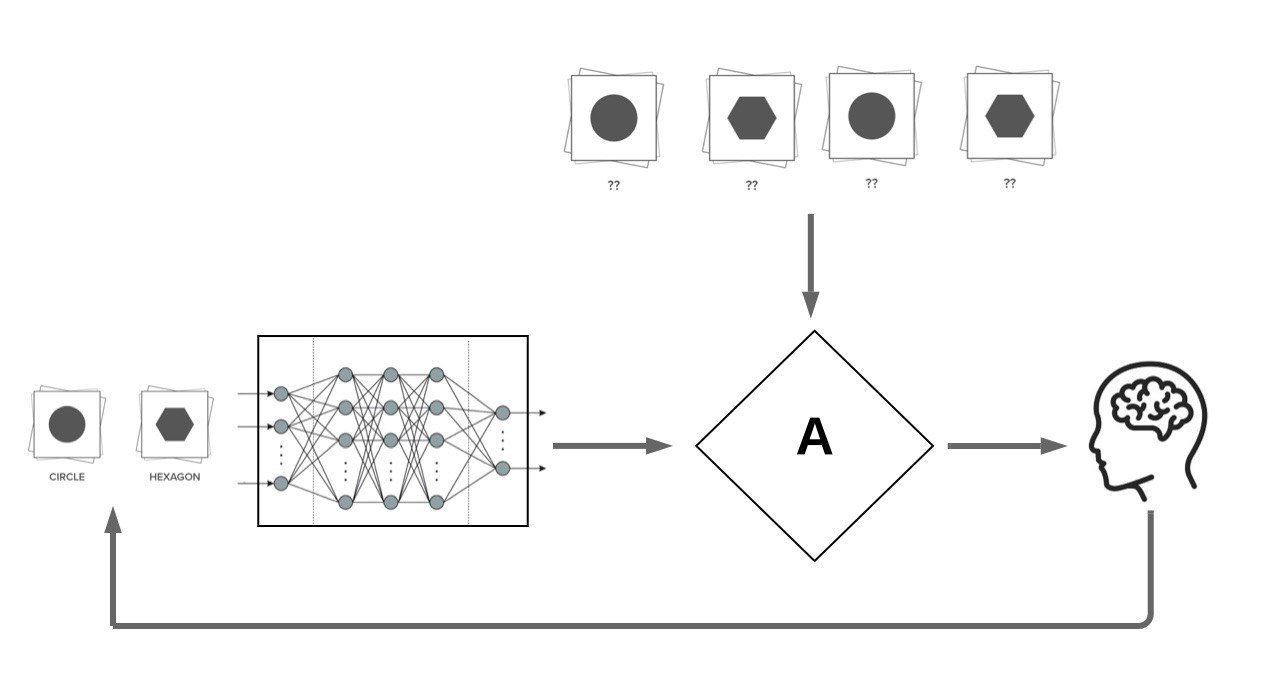
Active Learning
Active learning: reducing the required amount of labelled data in training ML models through allowing the model to "actively request for annotation of specific datapoints".
We focus on Pool Based Active Learning:
x^* = \argmax_{x \in \mathcal{U}}{A \left(x, f_{\mathcal{L}}, \mathcal{L}, \mathcal{U}\right)}
f_{\mathcal{L}}
\mathcal{U}
\mathcal{L}
x^*
x
(x^*, y^*)
AL Acquisition Functions
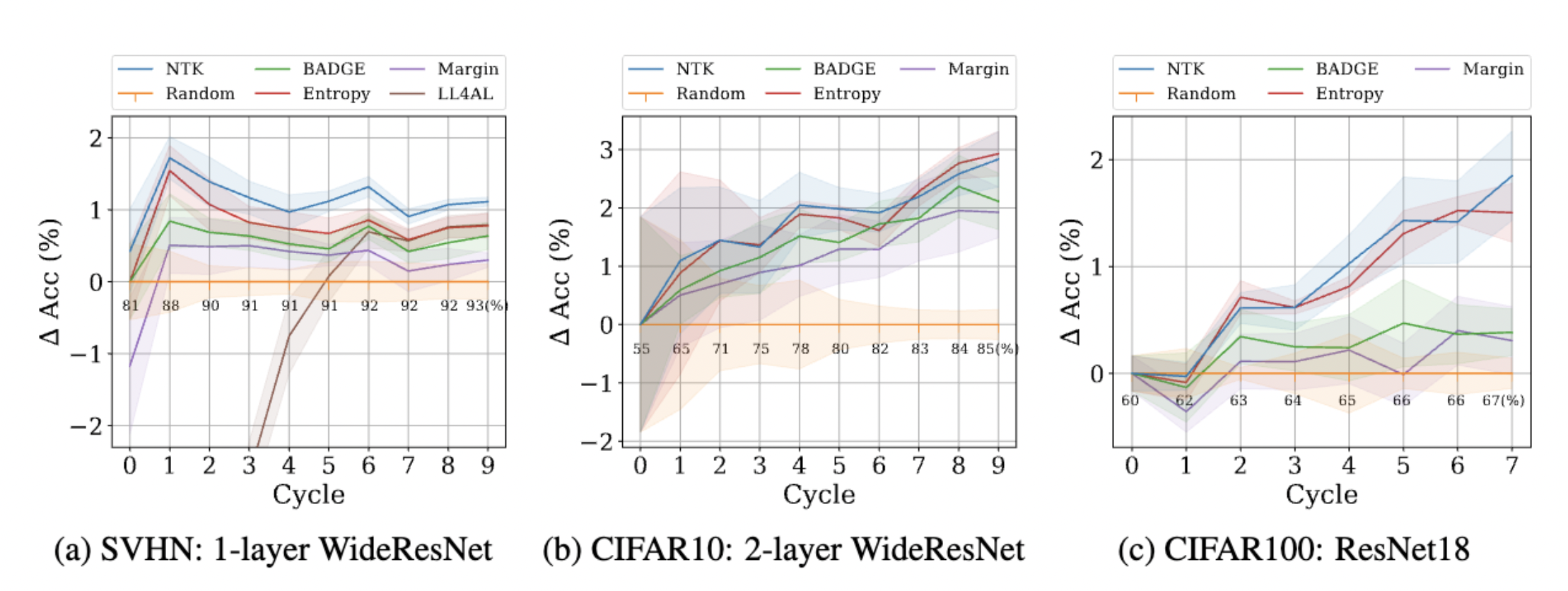
Most proposed acquisition functions in deep active learning can be categorized to two branches:
- Uncertainty Based: Maximum Entropy, BALD
- Representation-Based: BADGE, LL4AL
Our Motivation: Making Look-Ahead acquisition functions feasible in deep active learning:
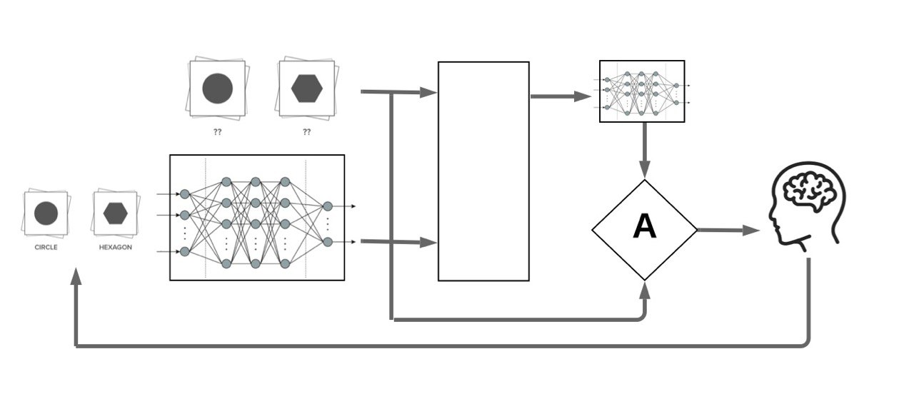
x
f_{\mathcal{L} \, \cup \, (x, \hat{y})}
\mathcal{L}
f_{\mathcal{L}}
x^*
(x^*, y^*)
Retraining
Engine
\mathcal{U}
Contributions
-
Problem: Retraining the neural network with every unlabelled datapoint in the pool using SGD is practically infeasible.
-
Solution: We propose to use a proxy model based on the first-order Taylor expansion of the trained model to approximate this retraining.
-
Contributions:
- We prove that this approximation is asymptotically exact for ultra wide networks.
- Our method achieves similar or improved performance than best prior pool-based AL methods on several datasets.
-
Our proxy model can be used to perform fast Sequential Active Learning (no SGD needed)!
Approximation of Retraining
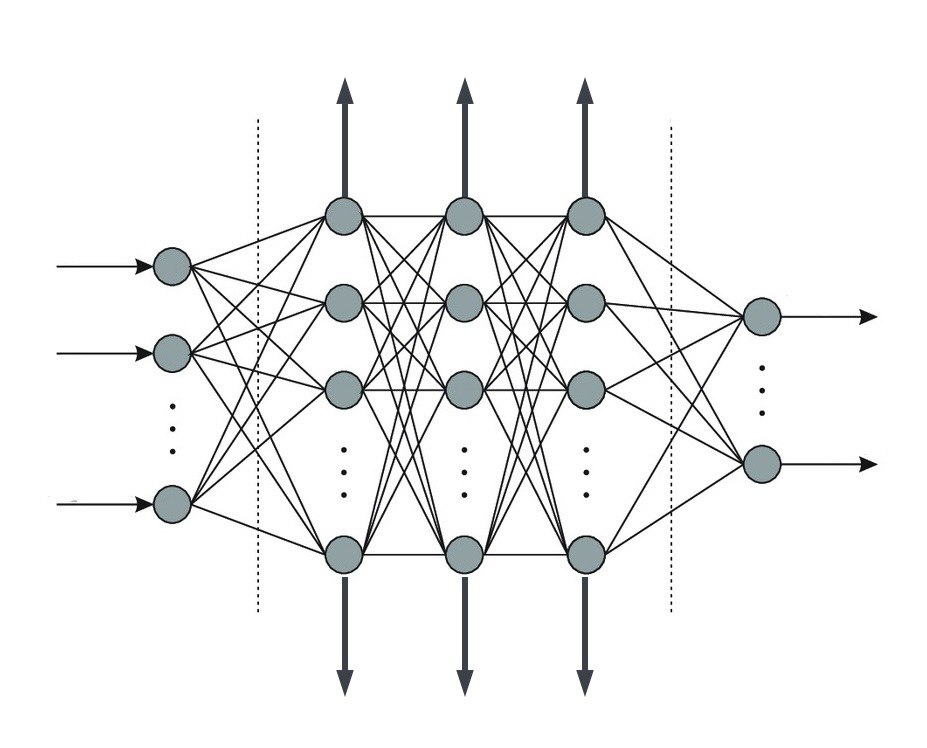
- Jacot et al.: training dynamics of suitably initialized infinitely wide neural networks can be captured by the Neural Tangent Kernels (NTKs).
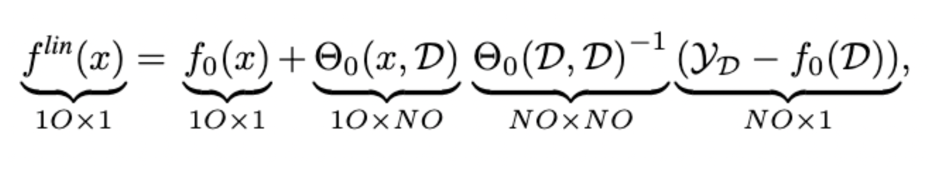
f^\textit{lin}_{\mathcal{L}}(x) = \, f_0(x) + \Theta_0(x, \mathcal{X})
\, {\Theta_0(\mathcal{X}, \mathcal{X})}^{-1}
(\mathcal{Y} - f_0(\mathcal{X}))
- Lee et al.: the first-order Taylor expansion of a neural network around its initialization has training dynamics converging to that of the neural network as the width grows:
\Theta_0(x, y) \vcentcolon= \nabla_{\theta} f_{0}(x) \, \nabla_{\theta} f_{0}(y)^\top
\infty
- Idea: approximate the retrained neural network on a new datapoint ( ) using the first-order taylor expansion of the network around the current model.
f_{\mathcal{L} \, \cup \, (x, \hat{y})}
f_{\mathcal{L}}
f_{\mathcal{L}^+}(x)
\approx f^\textit{lin}_{\mathcal{L}^+}(x)
=
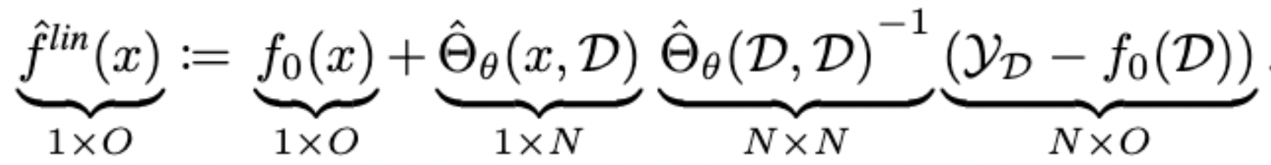
f_\mathcal{L}(x) + \Theta_{\mathcal{L}}(x, {\color{blue}{\mathcal{X}}}^{\color{orange}{+}}){\Theta_{\mathcal{L}}({\color{blue}{\mathcal{X}}}^{\color{orange}{+}}, {\color{blue}{\mathcal{X}}}^{\color{orange}{+}})}^{-1} \left (\mathcal{Y}^+ - f_\mathcal{L}(\mathcal{X}^+) \right )
+
-1
-
(
)
\times
f^\textit{lin}_{\mathcal{L}^+}(x) =
- We prove that this approximation is asymptotically exact for ultra wide networks and is empirically comparable to SGD for finite width networks.
Approximation of Retraining
Look-Ahead Active Learning
- We employ the proposed retraining approximation in a well-suited acquisition function which we call the Most Likely Model Output Change (MLMOC):
A_\textit{MLMOC}(x', f_{\mathcal L}, \mathcal{L}_t,\, \mathcal{U}_t)
\vcentcolon=
\sum_{x \in \mathcal{U}} \lVert f_{\mathcal L}(x) - f^\textit{lin}_{\mathcal L^+}(x)) \rVert_2
-
Although our experiments in the pool-based AL setup were all done using MLMOC, the proposed retraining approximation is general.
- We hope that this enables new directions in deep active learning using the look-ahead criteria.
Experiments
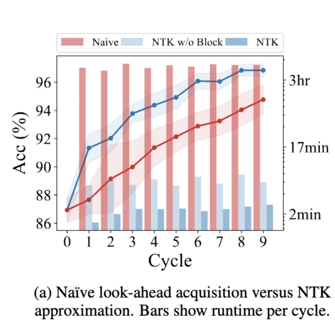
Retraining Time: The proposed retraining approximation is much faster than SGD.
Experiments: The proposed querying strategy attains similar or better performance than best prior pool-based AL methods on several datasets.
A Fast, Well-Founded Approximation to the Empirical Neural Tangent Kernel
The Neural Tangent Kernel
-
Has enabled lots of theoretical insights into deep NNs:
- Studying the geometry of the loss landscape of NNs (Fort et al. 2020)
- Prediction and analyses of the uncertainty of a NN’s predictions (He et al. 2020, Adlam et al. 2020)
-
Has been impactful in diverse practical settings:
- Predicting the trainability and generalization capabilities of a NN (Xiao et al. 2018 and 2020)
- Neural Architecture Search (Park et a. 2020, Chen et al. 2021)
- *Your work here* :D
eNTK: Computational Cost
-
Is, however, notoriously expensive to compute :(
- Both in terms of computational complexity, and memory complexity!
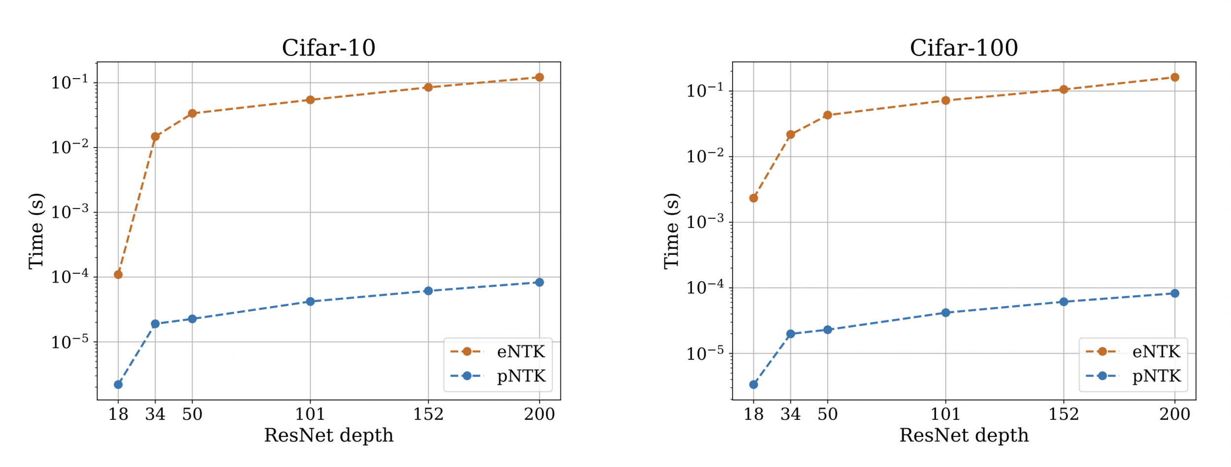
- Computing the Full empirical NTK of ResNet18 on Cifar-10 requires over 1.8 terabytes of RAM !
-
This work:
- An approximation to the ENTK, dropping the O term from the above equations!
\underbrace{\Theta_f(X_1, X_2)}_{N_1 O \times N_2 O} = \underbrace{J_\theta f(X_1)}_{N_1 \times O \times P} \otimes \underbrace{{J_\theta f(X_2)}^\top}_{P \times O \times N_2}
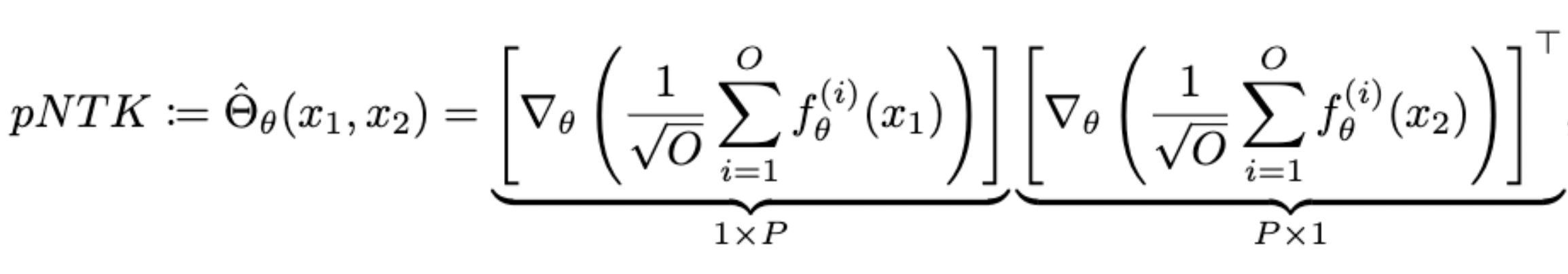
pNTK: An Approximation to the eNTK
- For each NN, we define pNTK as follows:
(We are basically adding a fixed untrainable dense layer at the end of the neural network!)
- Computing this approximation requires O(O^2) less time and memory complexity in comparison to the eNTK. (Yay!)
Computational Complexity: pNTK vs eNTK
pNTK: An Approximation to the eNTK
- Previous work already implies that for infinitely wide NNs at initialization, pNTK converges to the eNTK. In the infinitely wide regime, the eNTK of two datapoints is a diagonal matrix.
- Lots of recent papers have used the same property, but with little to no justification!
- We show that although this property is not valid in the finite width regime, it converges to the eNTK as width grows.
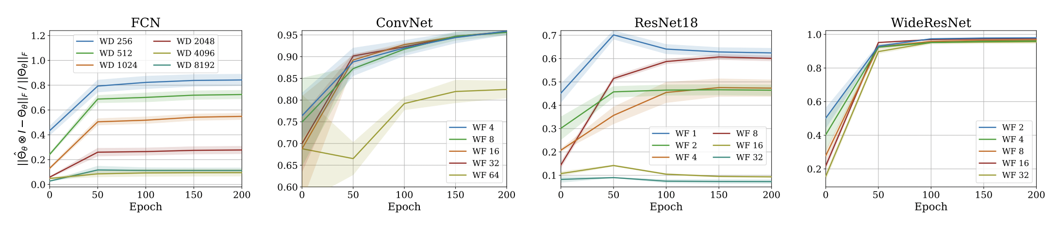
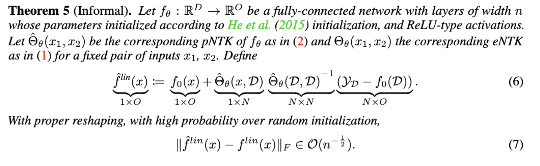
Approximation Quality: Frobenius Norm
- Why?
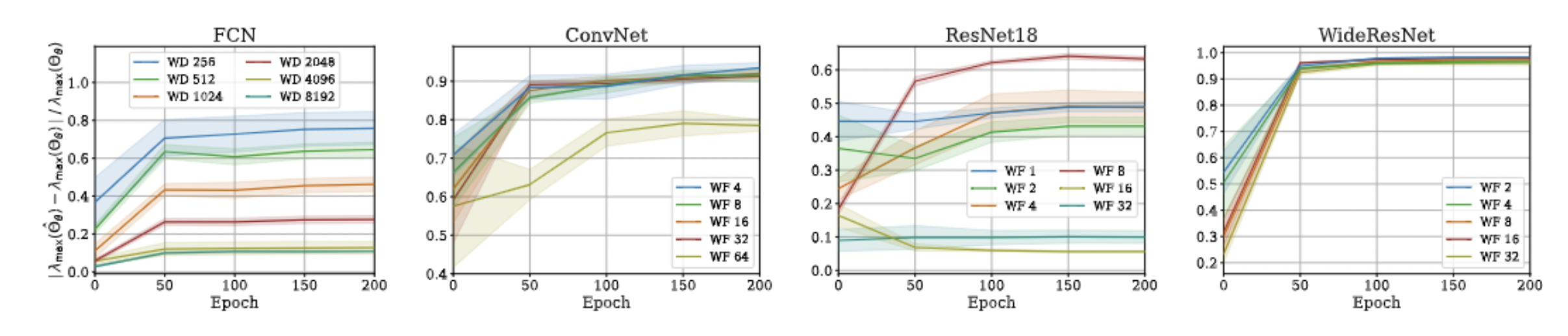
- The diagonal elements of the difference matrix grow linearly with width
- The non-diagonal elements are constant with high probability
- Frobenius Norm of the difference matrix relatively converges to zero
\sim
Approximation Quality: Frobenius Norm
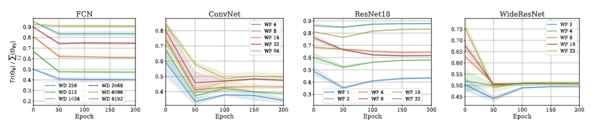
Approximation Quality: Eigen Spectrum
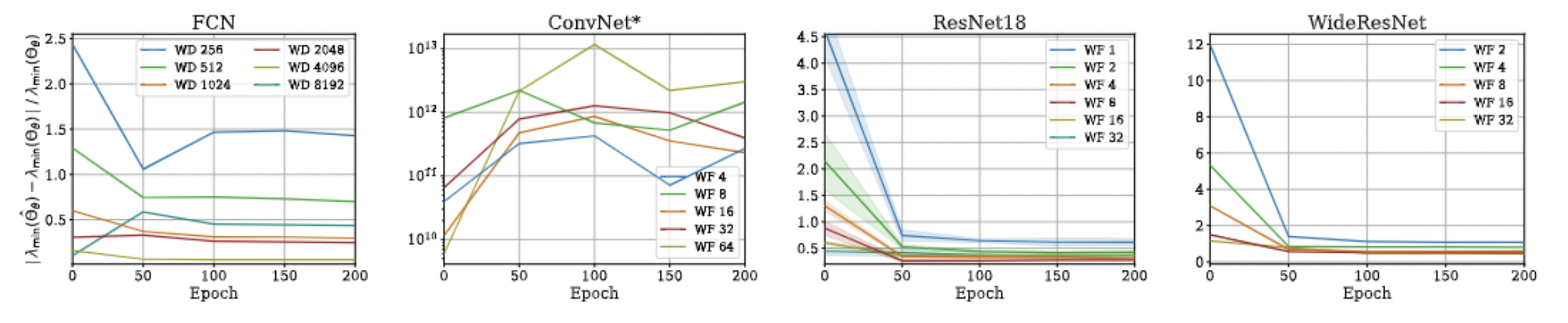
- Proof is very simple!
- Just a triangle inequality based on the previous result!
- Unfortunately, we could not come up with a similar bound for min eigenvalue and correspondingly the condition number, but empirical evaluations suggest that such a bound exists!
\sim
Approximation Quality: Eigen Spectrum
Approximation Quality: Kernel Regression
- Note that pNTK is a scalar-valued kernel, but the eNTK is a matrix-valued kernel!
- Intuitively, one might expect that they can not be used in the same context for kernel regression.
- But, there's a work-around, as this is a well known problem:
Approximation Quality: Kernel Regression
- Note: This approximation will not hold if there is any regularization (ridge) in the kernel regression! :(
- Note that we are not scaling the function values anymore!
\sim
Approximation Quality: Kernel Regression
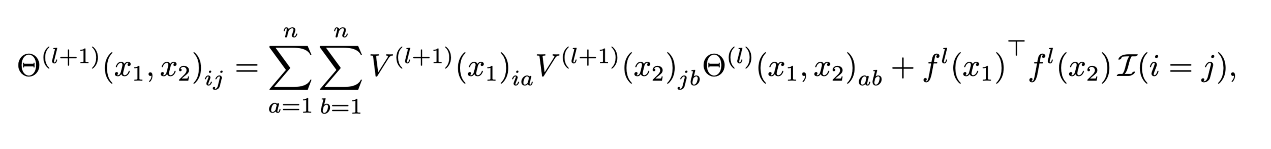
Proof Idea:
- Start with layer 1, derive bounds for elements of the empirical tangent kernel (diagonal)
- Recursively derive bounds for elements of next layer:
- Why Standard Parameterization?
- Optimizing different architectures with NTK-parameterization was hard!
- Any surprise?
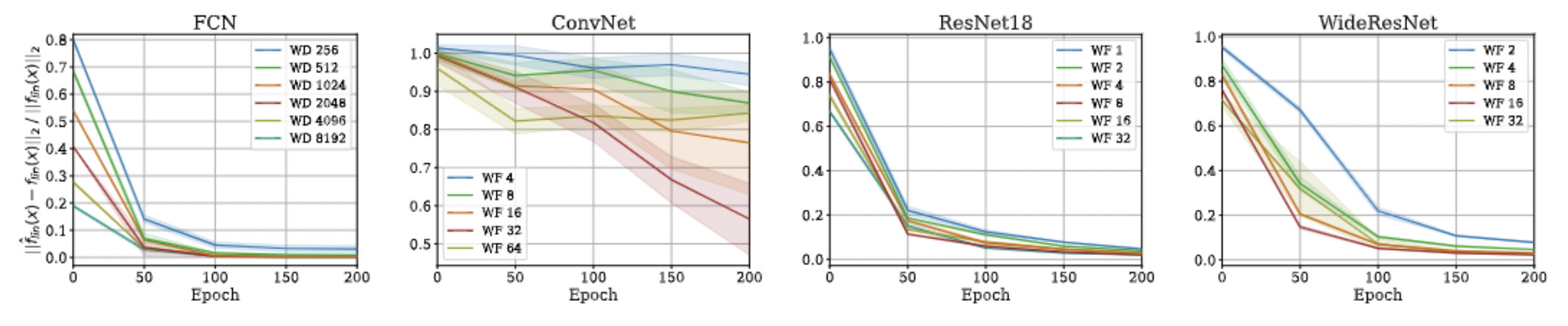
- As training goes on, local linearization becomes more exact in terms of test accuracy. (not really a surprise! :p)
More recent stuff
-
Growing width of the neural networks.
- ResNets typically grow in width as depth grows (in each block).
- Not much analysis out there on the impact of shrinking/growing width with depth.
- MuP: This kind of growing width would result in a scaled parameter update after each gradient step.
- Idea: Can we remove the growing width and still attain the same performance?
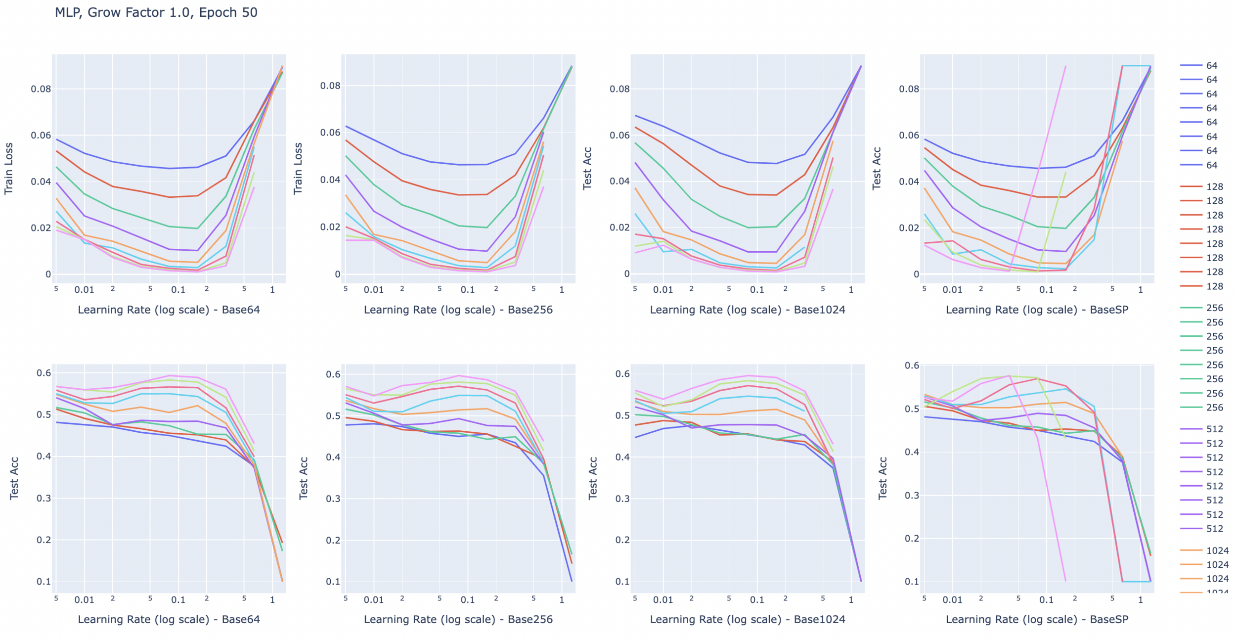
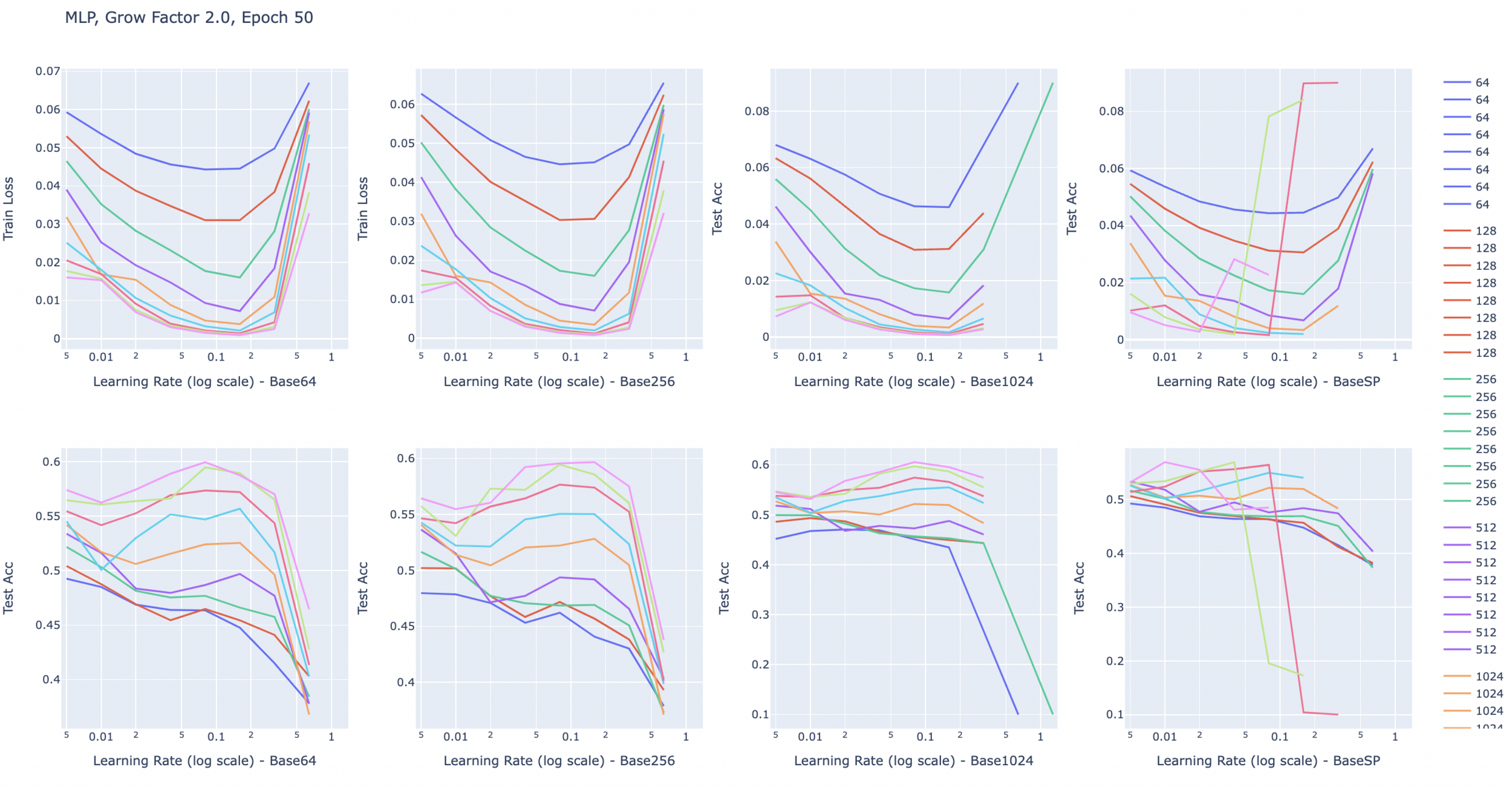
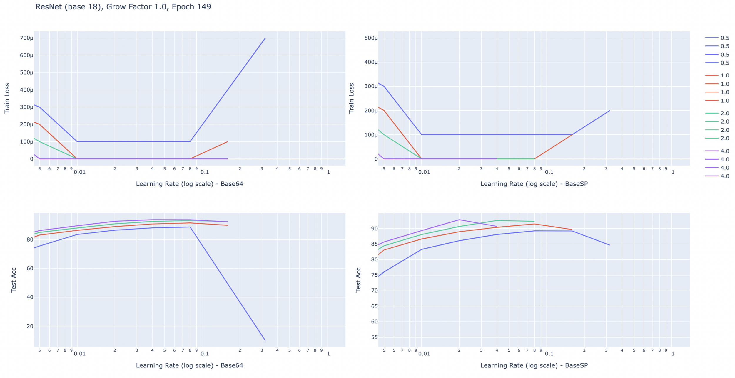
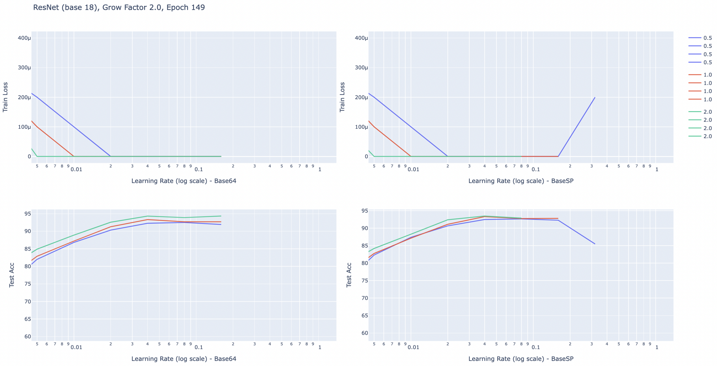
Results for now
- Found a ResNet18 variant with 2.4m parameters that attains the same performance (generalization) on Cifar10, SVHN and FashionMNIST.
- Results partly extend to ImageNet and bigger ResNets
- New analyses in progress....
Thanks!
Hello!
By Amin Mohamadi


