Probabilistic Modeling and Analysis
for Cosmology
Andreas Tersenov
29 January 2026


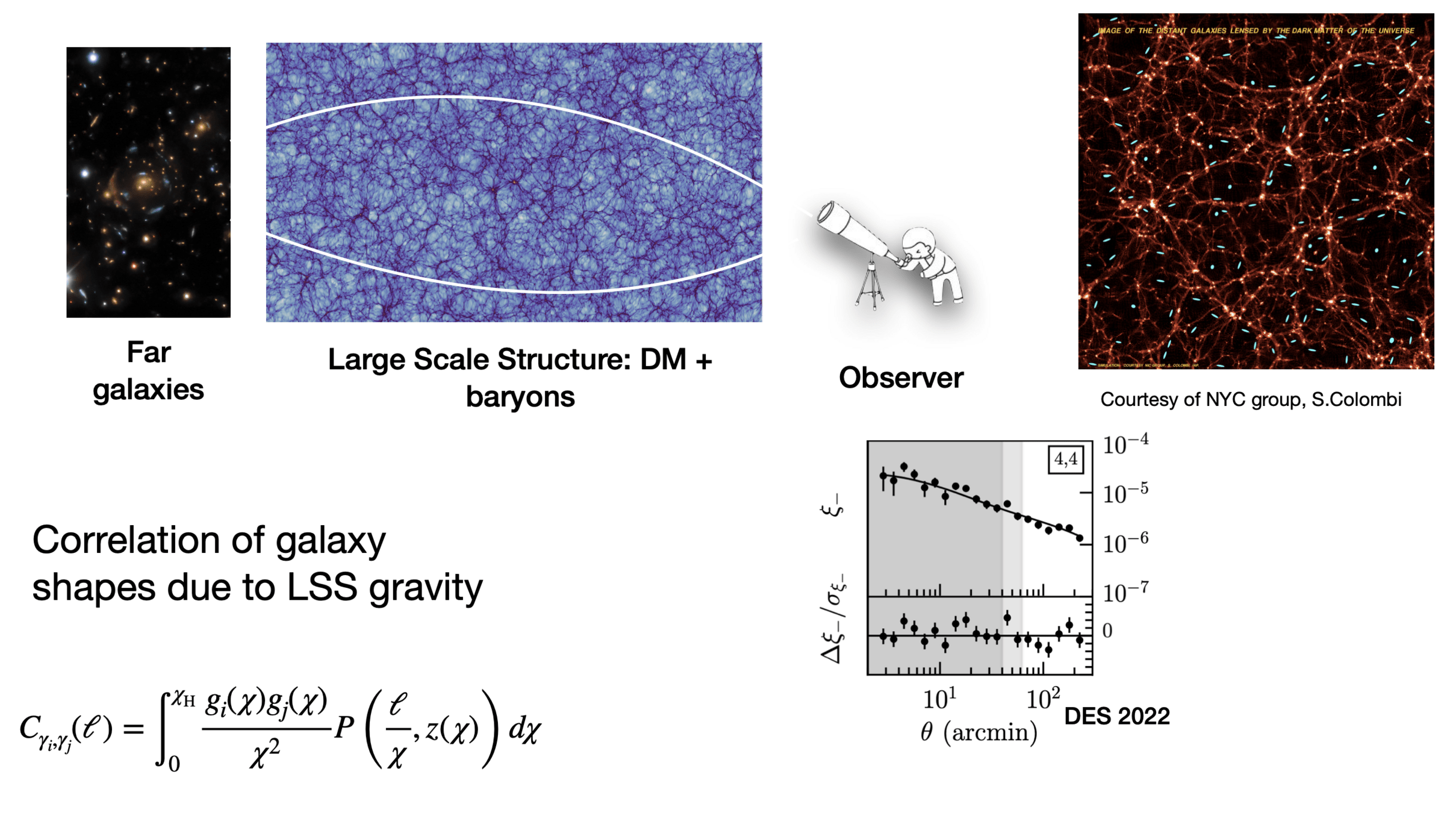
Background: Weak Lensing Analysis
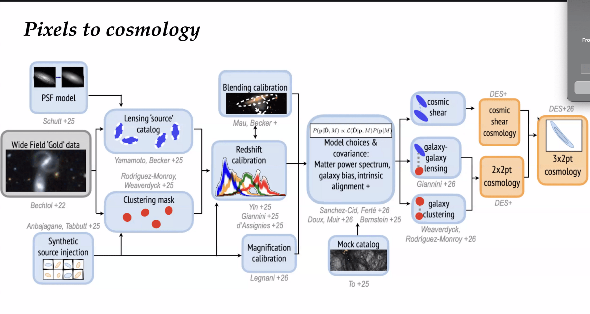
An End-to-End approach: From Pixel-Level Reconstruction to Robust Cosmology
The Data/Pixels
-
Catalogues: shear calibration, masks, blinding, tomography...
-
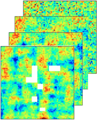
Mass Mapping: Inverse problems, PnPMass, Denoising.
-
Methods: DL Priors, Convex Optimization.
The Signal & Physics
-
Summary Statistics: 2pt, HOS (Peaks, PDF, l1-norm)
-
Systematics: Baryonic Feedback, IA, Masks, Noise.
-
Theory: Large Deviation Theory validation, Euclid paper on theory HOS.
The Inference
-
Methodology: Simulation-Based Inference (SBI) & Explicit Inference.
-
Computational Core: JAX ecosystem, Differentiable Programming, Samplers, ML-emulators.
Differentiable pipelines (JAX/PyTorch), ML/DL, probabilistic programming (NumPyro), advanced sampling, neural density estimation, ML/DL for scientific inference, and the diagnosis of model misspecification
Impact of Mass Mapping on Cosmology Inference
Weak Lensing Mass Mapping
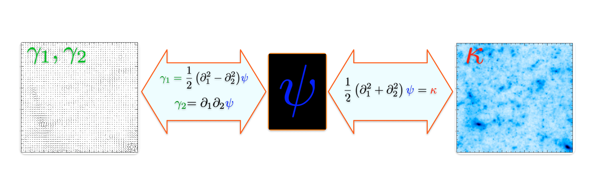
- From convergence to shear:
- From shear to convergence:
\gamma_i = \hat{P}_i \kappa
\kappa = \hat{P}_1 \gamma_1 + \hat{P}_2 \gamma_2
Mass mapping is an ill-posed inverse problem
Different algorithms have been introduced, with different reconstruction fidelities
But... does the choice of the mass-mapping algorithm have an impact on the final inferred cosmological parameters?
Or as long as you apply the same method to both observations and simulations it won't matter?
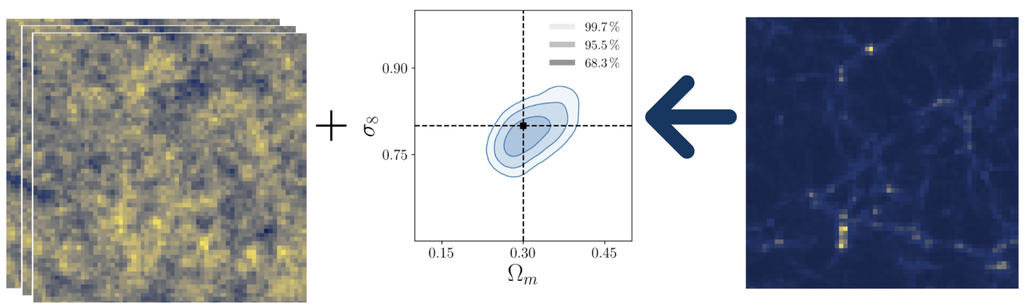
For which we have/assume an analytical likelihood function
x
t = f(x)
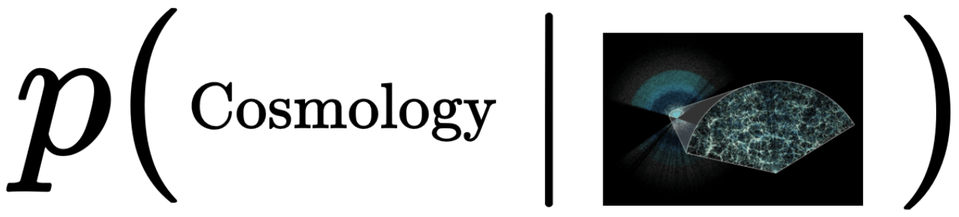
How to constrain cosmological parameters?
Likelihood → connects our compressed observations to the cosmological parameters
\underbrace{p\left(\theta \mid t=t_0\right)}_{\text {posterior }} \propto \underbrace{p\left(t=t_0 \mid \theta\right)}_{\text {likelihood }} \underbrace{p(\theta)}_{\text {prior }}
p\left(t=t_0 \mid \theta\right)
Credit: Justine Zeghal
2pt vs higher-order statistics
The traditional way of constraining cosmological parameters misses the non-Gaussian information in the field.

x
t = f(x)

DES Y3 Results
Credit: Justine Zeghal
Higher Order Statistics: Peak Counts
=
+
+
+
+
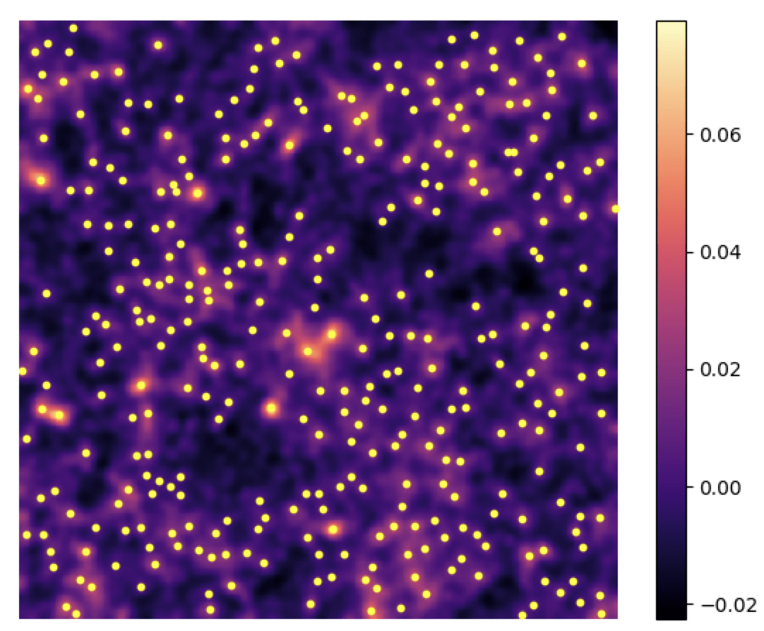
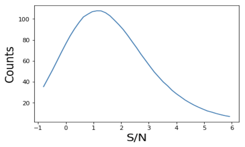
- Peaks: local maxima of the SNR field
- Peaks trace regions where the value of 𝜅 is high → they are associated to massive structures
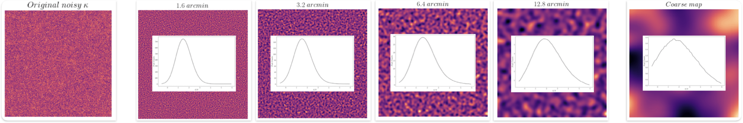
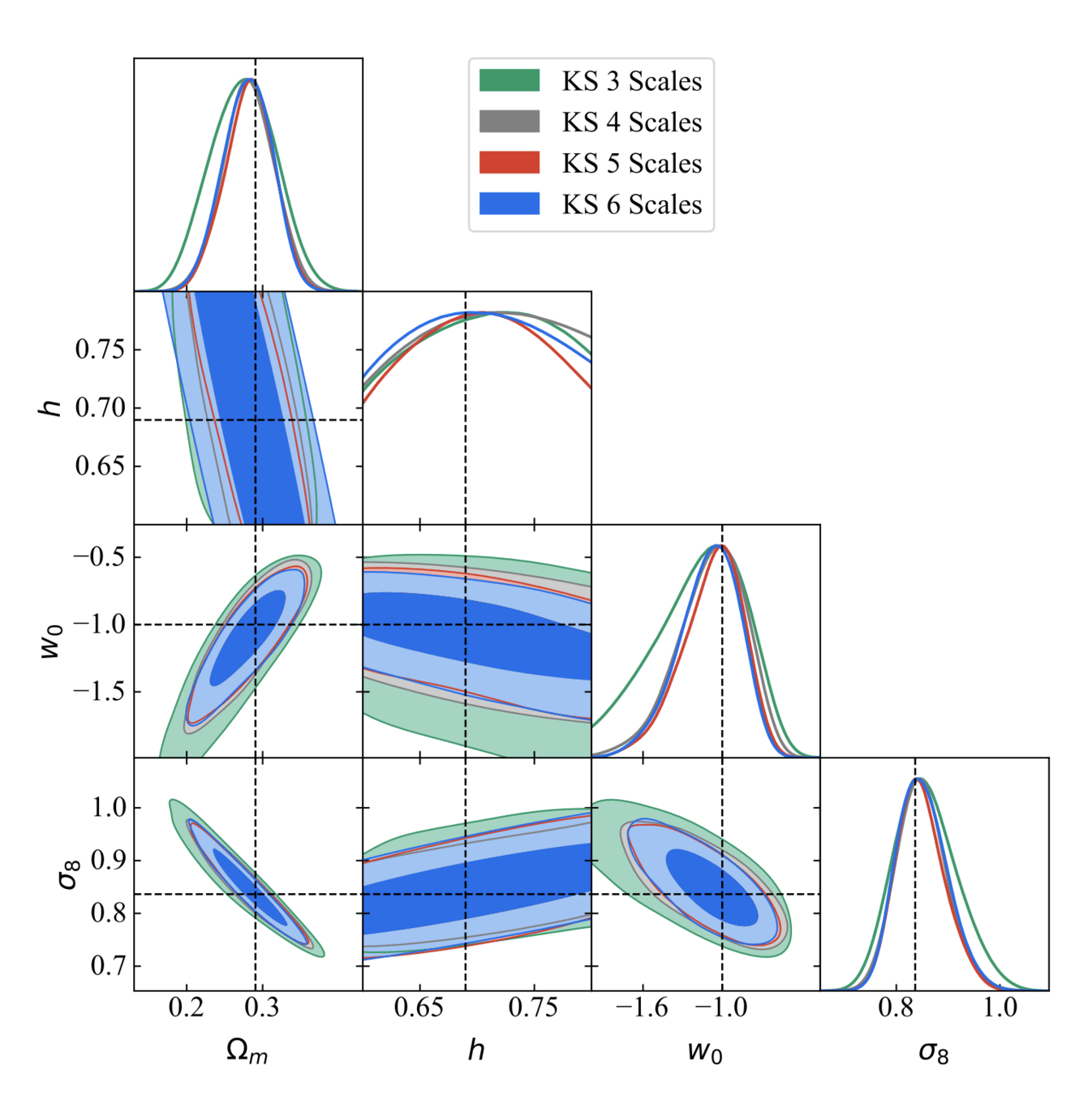
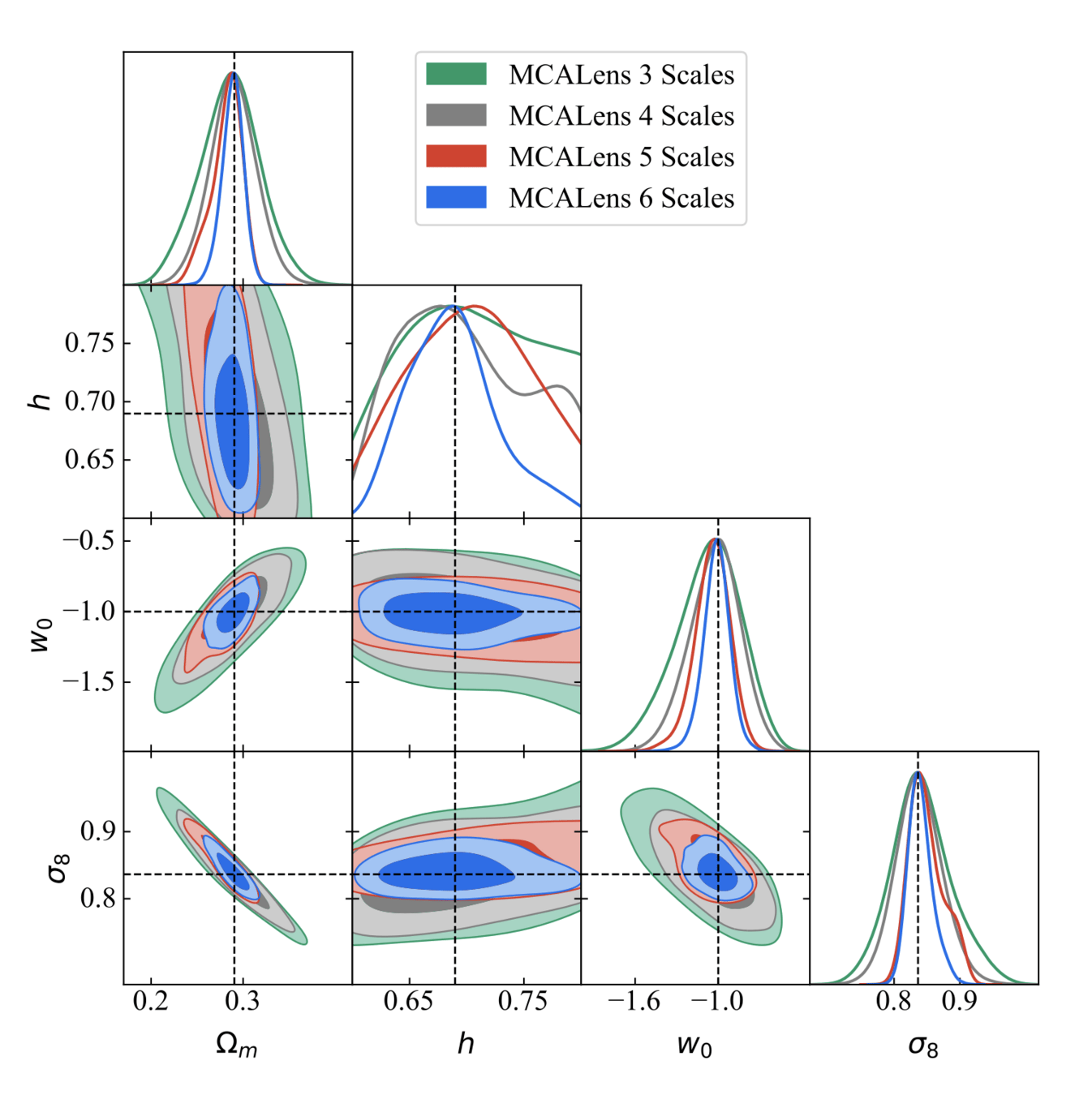
Multi-scale (wavelet) peak counts
Ajani et. al 2021
cosmoSLICS pipeline
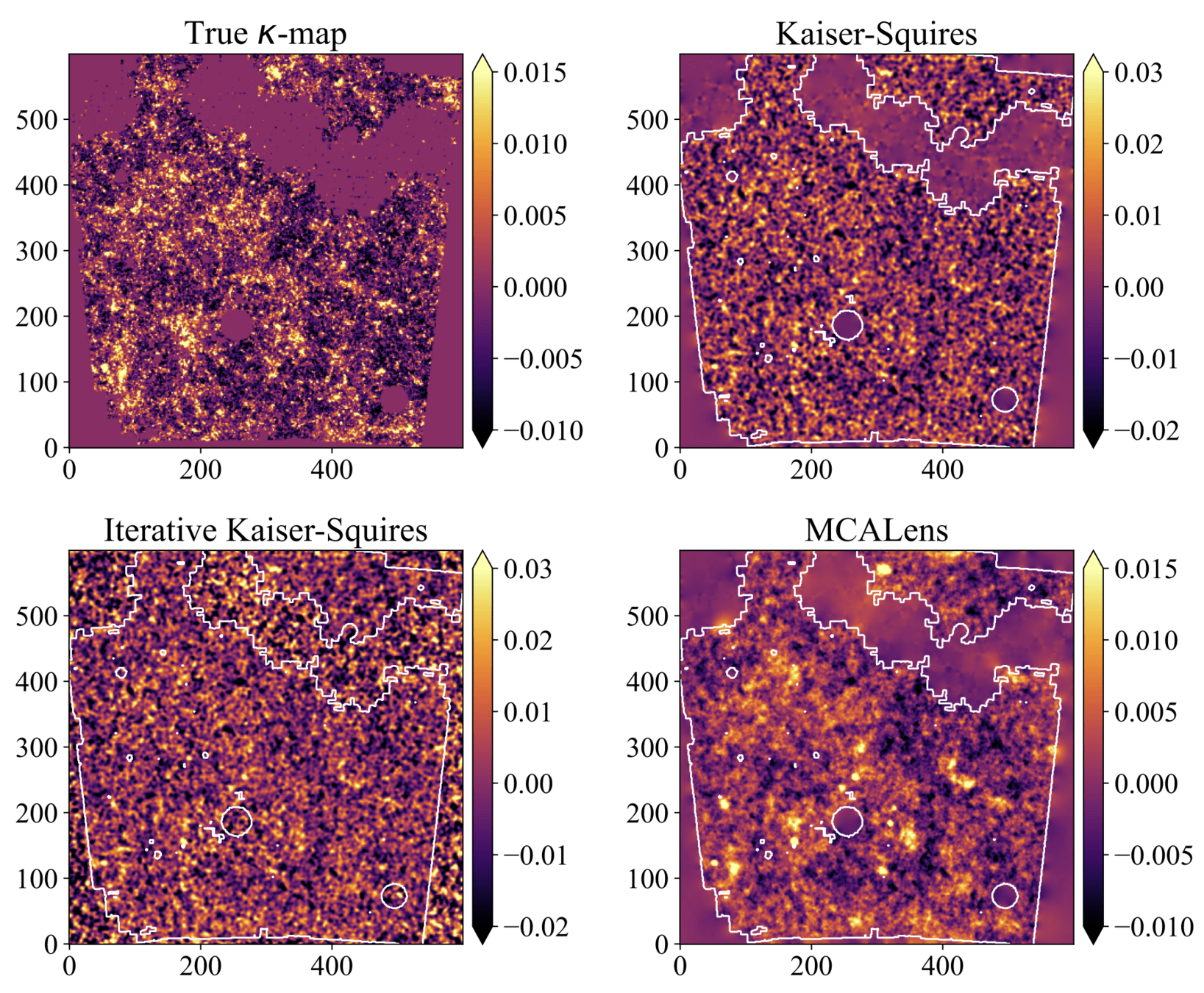
\begin{array}{ll}
\hline \hline
\text{Method} & \text{RMSE} \downarrow \\
\hline
\text{KS } & 1.1 \times 10^{-2} \\
\text{iKS } & 1.1 \times 10^{-2} \\
\text{MCALens} & 9.8 \times 10^{-3} \\
\hline
\end{array}
- Add realistic masks & Euclid-like noise to shear maps
- Use different algorithms for the mass mapping
- Compression with higher-order statistics (peaks)
- Gaussian Likelihood + MCMC
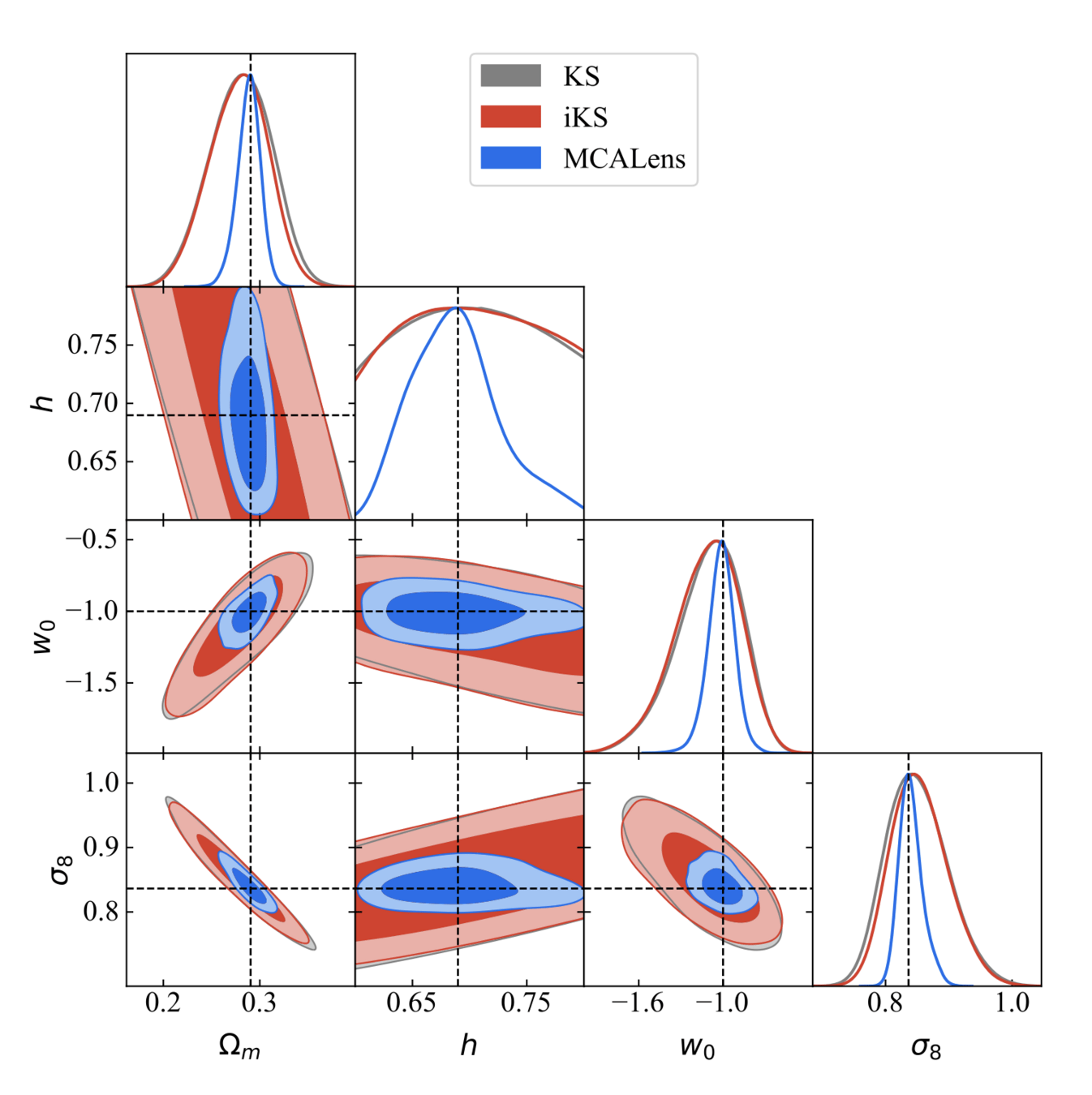
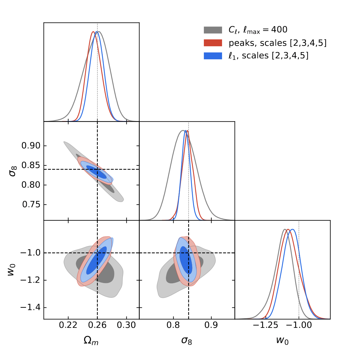
Results
Where does this improvement come from?
FoM improvement → 150%
Plug-and-Play Mass Mapping with Uncertainty Quantification
Deep Learning for Mass Mapping?
| Mass mapping method | Type | Accurate | Flexible | Fast rec. | Fast UQ |
|---|---|---|---|---|---|
| Iterative Wiener | Model-driven (Gaus. prior) | ✗ | ✓ | ✓ | ✗ |
| MCALens | Model-driven (Gaus. + sparse) | ≈ | ✓ | ✗ | ✗ |
| DeepMass | Data-driven (UNet) | ✓ | ✗* | ✓ | ✓ |
| DeepPosterior | Data-driven (UNet + MCMC) | ✓ | ✓ | ✗ | ✗ |
| MMGAN | Data-driven (GAN) | ✓ | ✗* | ≈ | ≈ |
| What we'd like | Data-driven | ✓ | ✓ | ✓ | ✓ |
Plug-and-Play Mass Mapping
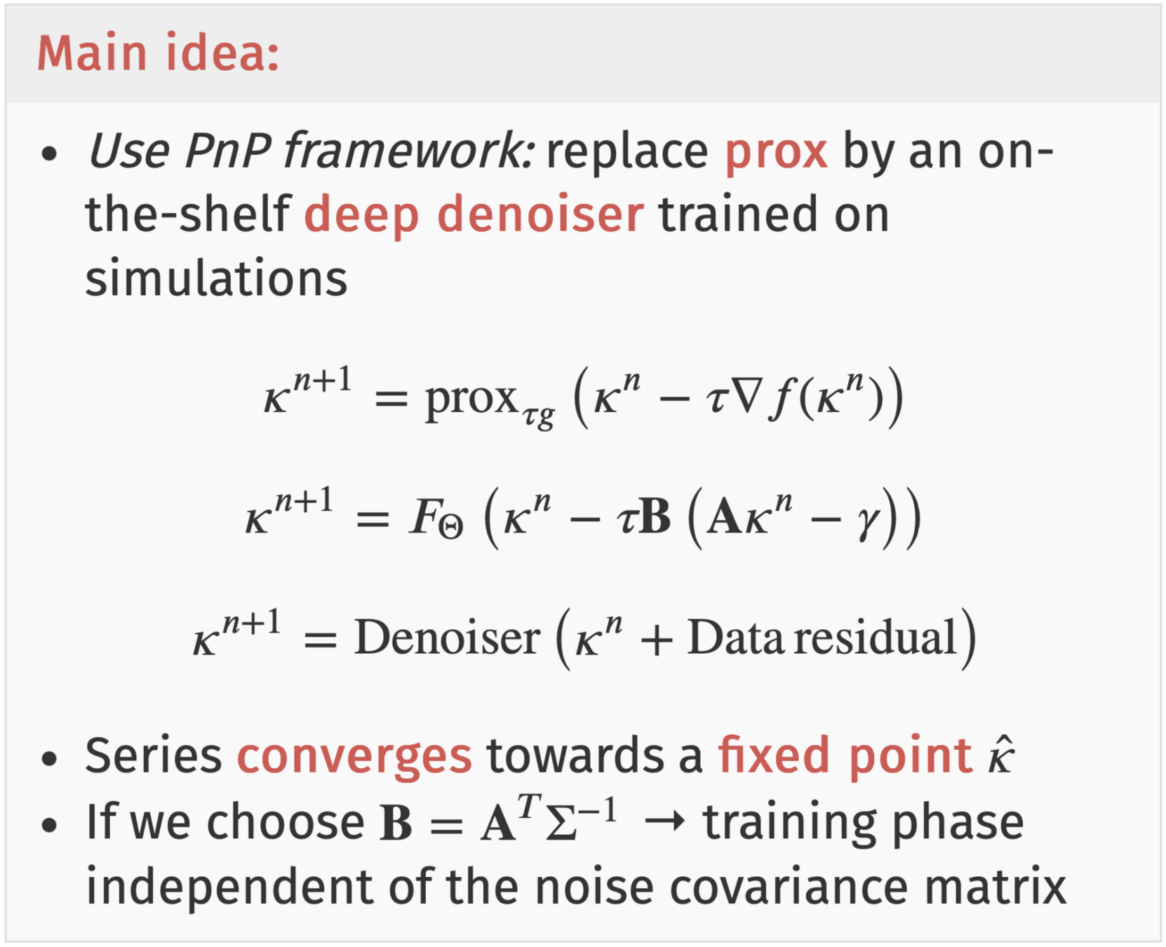
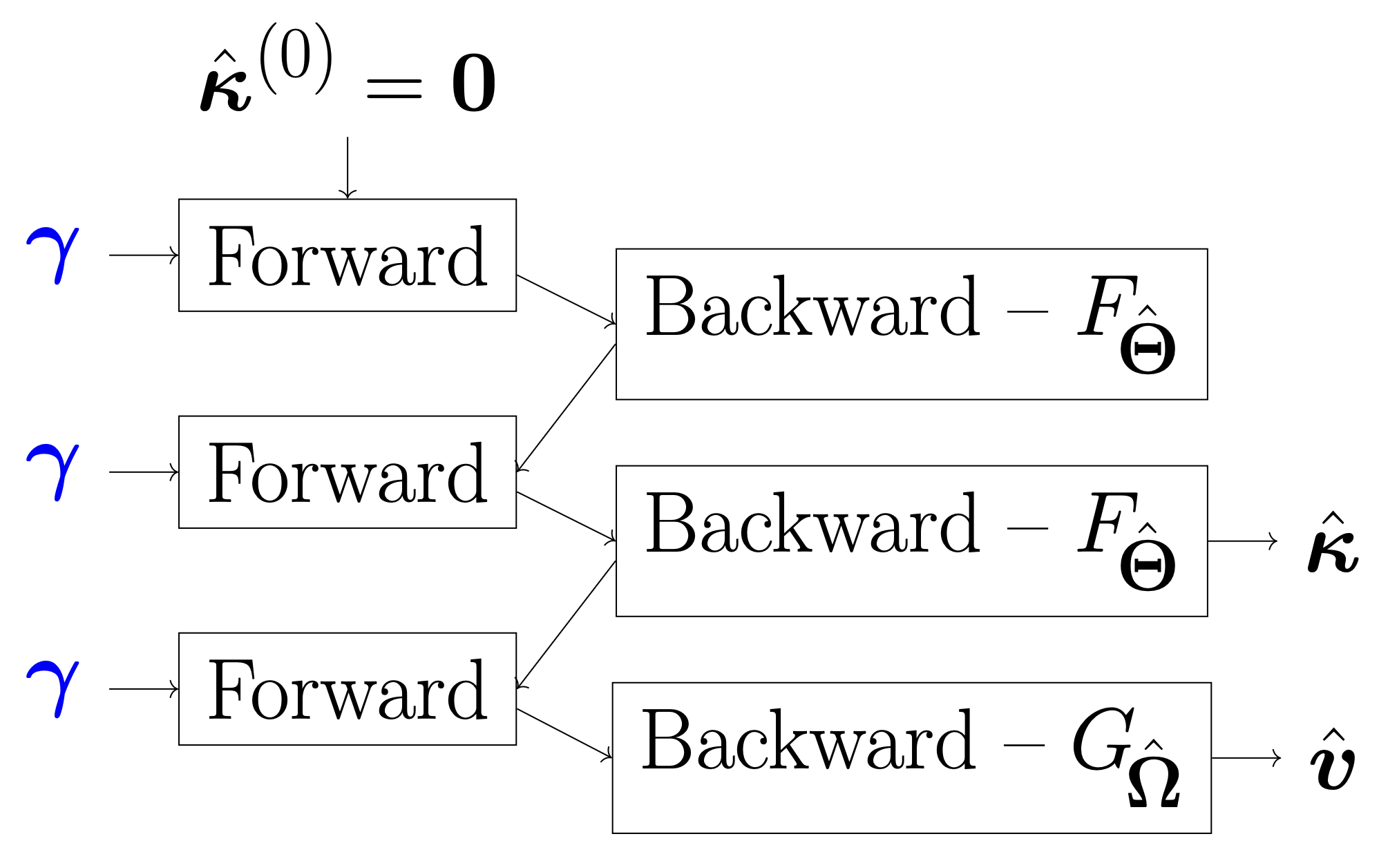
Instead of explicitly writing down a prior, we learn what a "likely" 𝜅 looks like from simulations and enforce it through denoising.
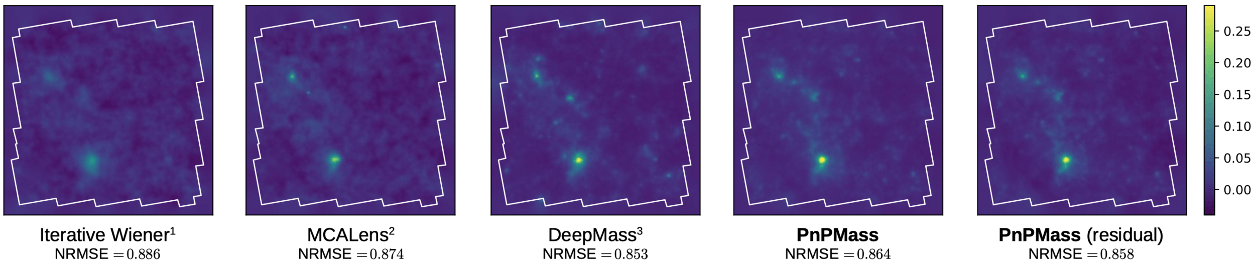
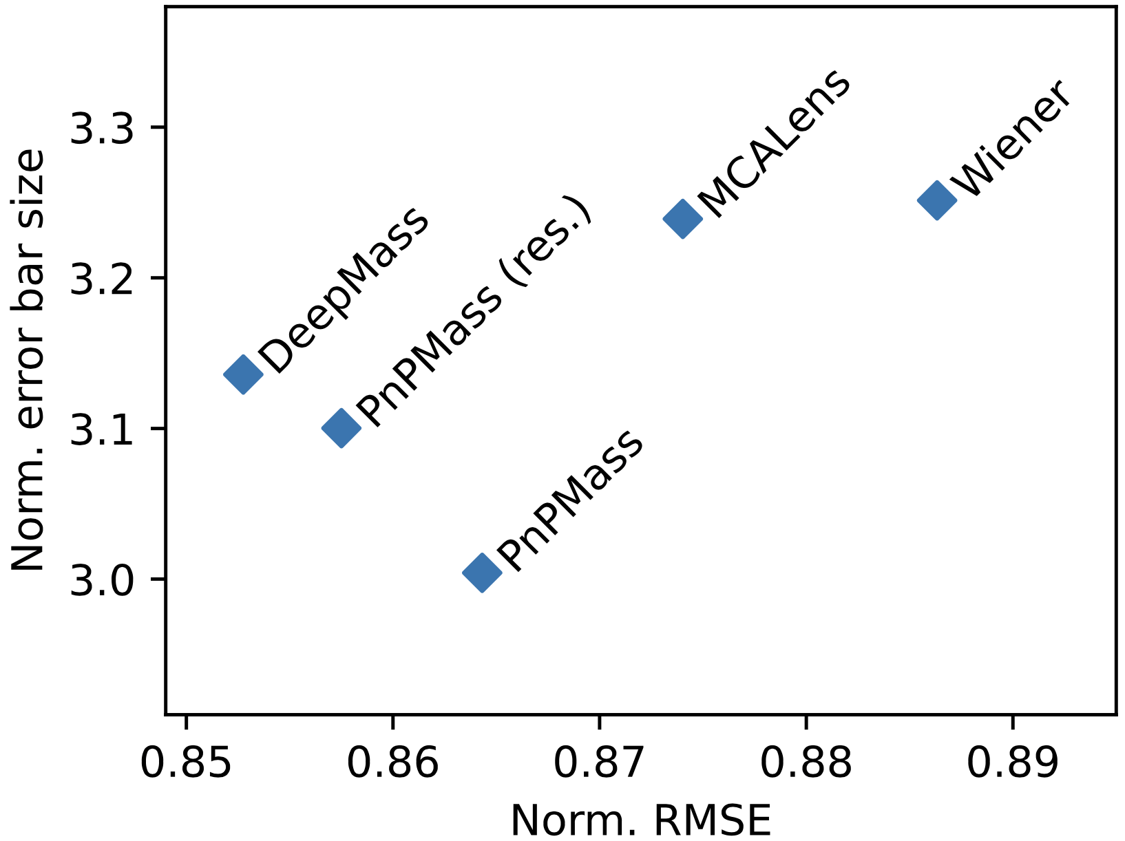
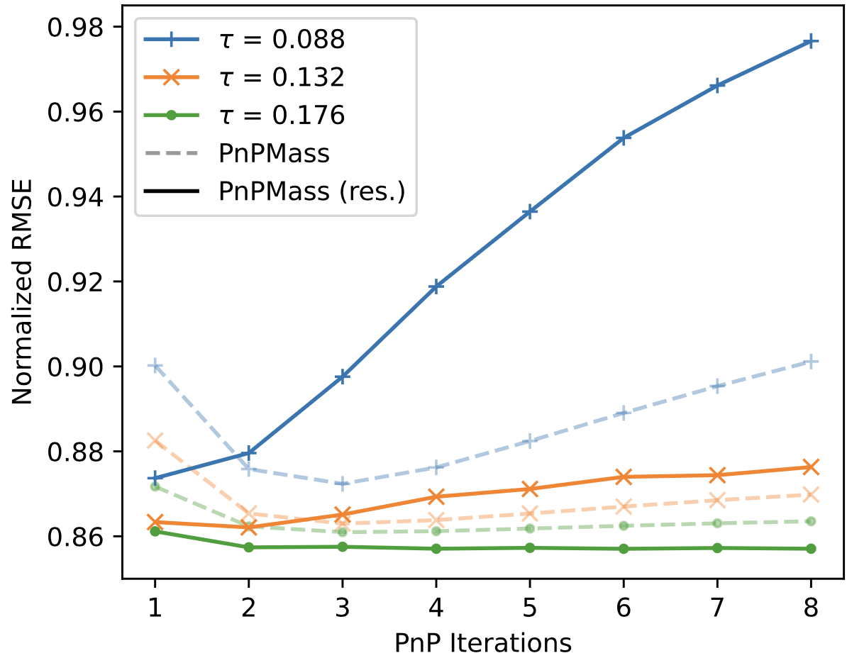
Results
Impact of baryonic effects on cosmology inference with HOS
Testing impact of baryonic effects on WL HOS
Idea - Explore two things:
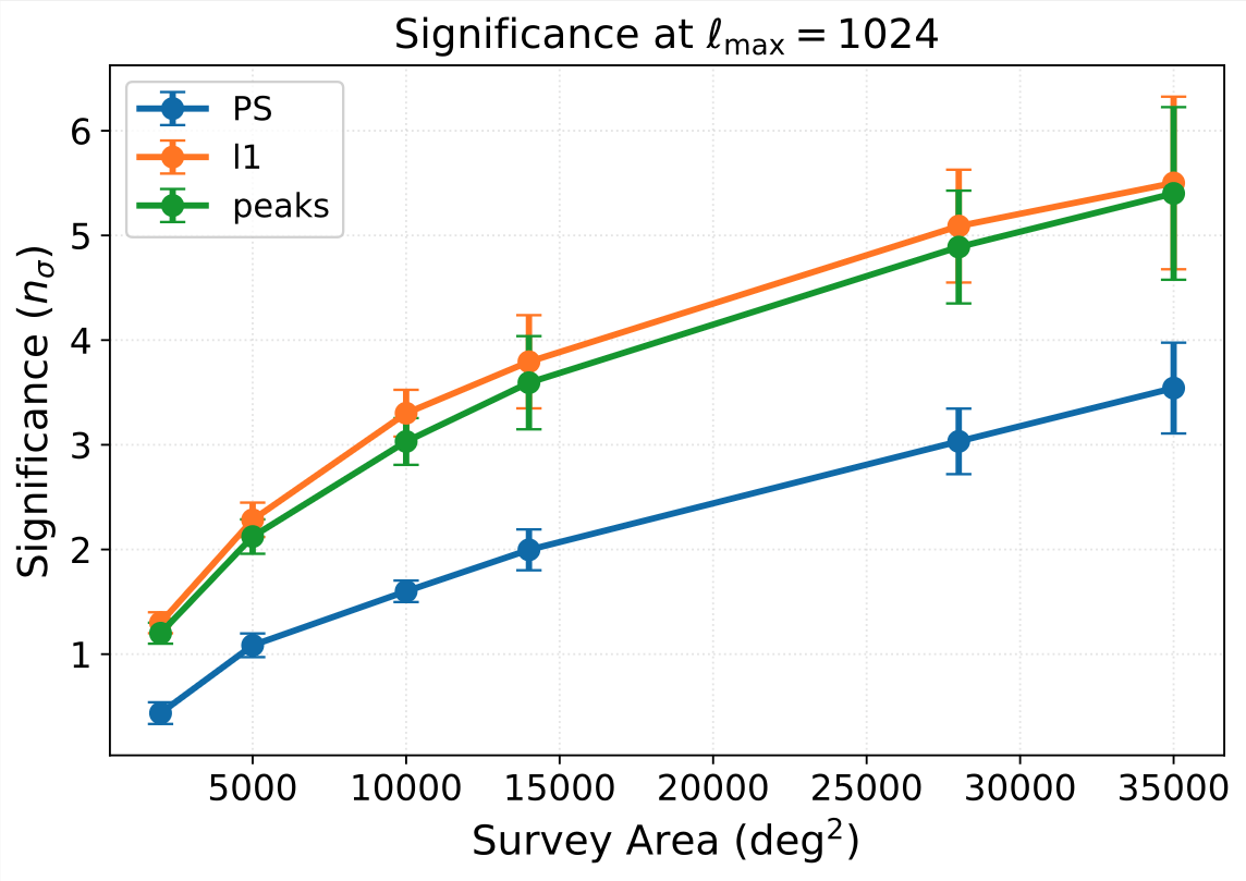
- Information content of summary statistics as a function of scale cuts & survey area
- Testing the impact of baryonic effects on posterior contours
This will show:
- On what range of scales can the different statistics be used without explicit model for baryons
- Answer the question: how much extra information beyond the PS these statistics can access in practice
Baryonic effects
- Effects that stem from astrophysical processes involving ordinary matter (gas cooling, star formation, AGN feedback)
-
They modify the matter distribution by redistributing gas and stars within halos.
-
Suppress matter clustering on small scales
- Depend on the cosmic baryon fraction and cosmological parameters.
-
Must be modeled/marginalized over to avoid biases in cosmological inferences from WL.
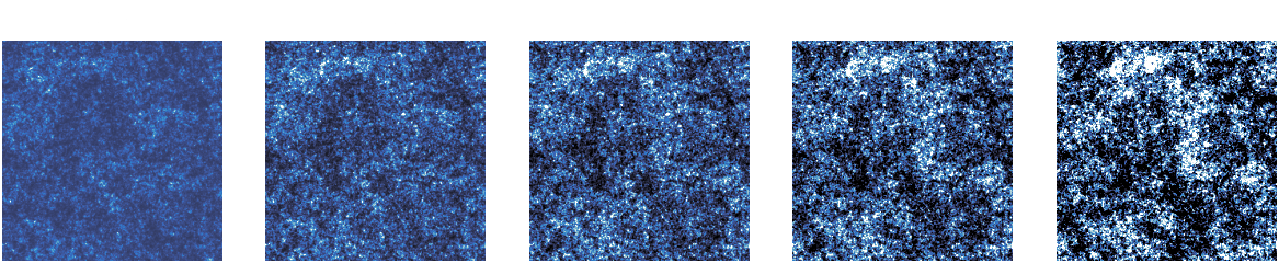
Baryonic impact on LSS statistics
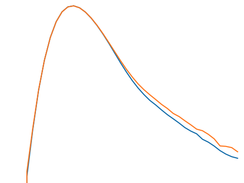
baryonic effects in P(k)
Credit: Giovanni Aricò
cosmoGRID simulations:
Power Spectrum
Wavelet l1-norm: sum
of wavelet coefficients
within specific amplitude
ranges across different
wavelet scales
Wavelet peaks: local maxima of wavelet
coefficient maps
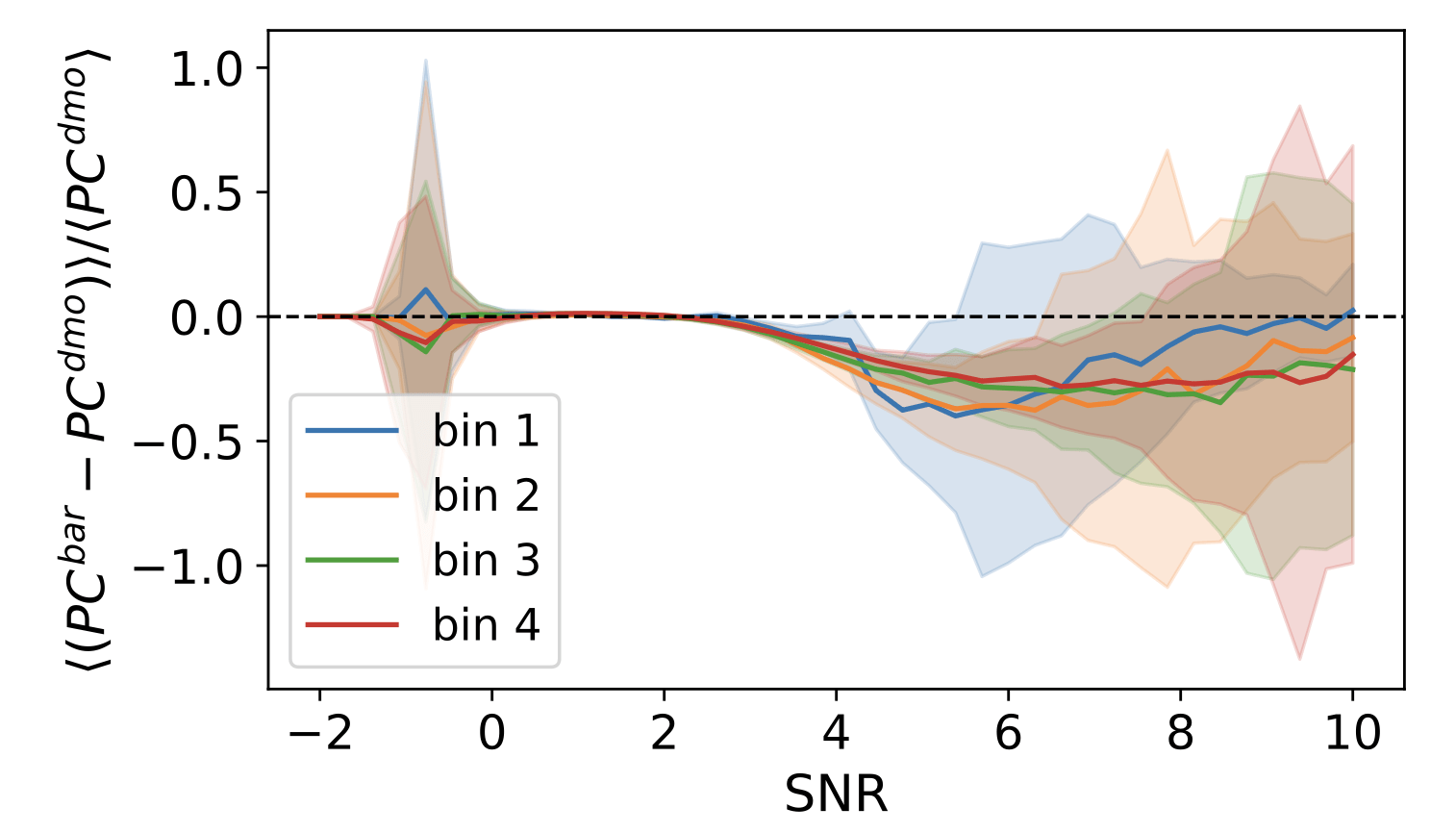
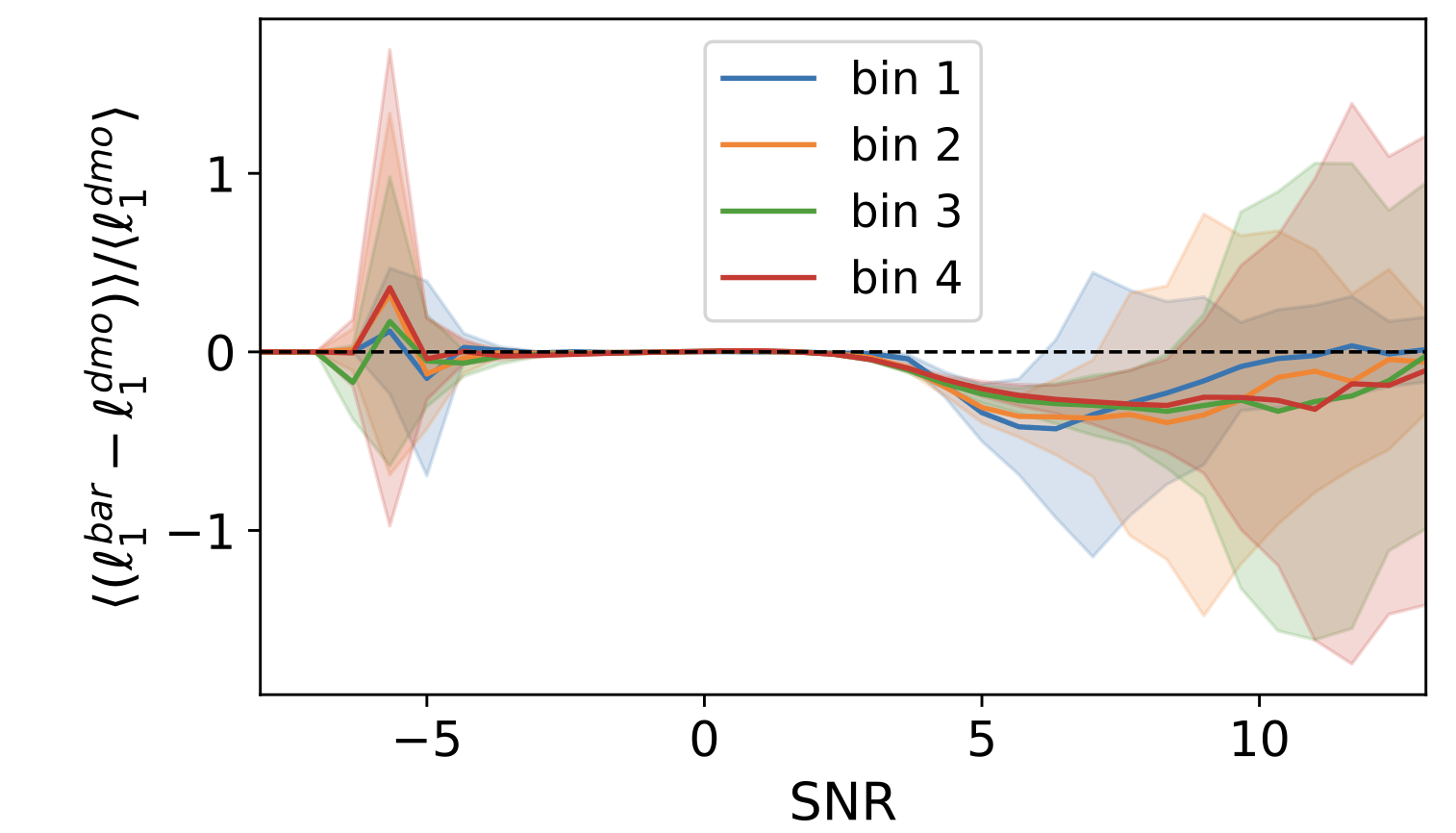
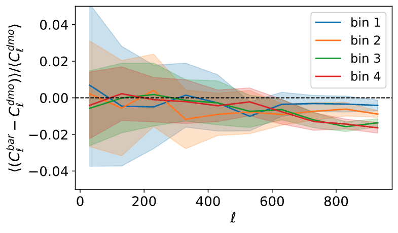
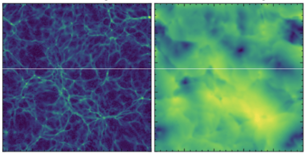
N-body sims, providing DMO and baryonified full-sky κ-maps from the same IC, for 2500 cosmologies. Baryonic effects are incorporated using a shell-based Baryon Correction Model (Schneider et. al 2019).
Inference method: SBI
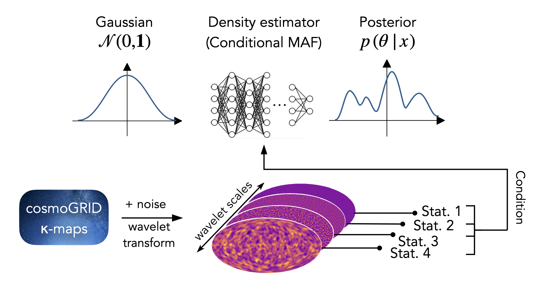
Training objective
\mathcal{L} = - \log p_\phi ( \theta | x )
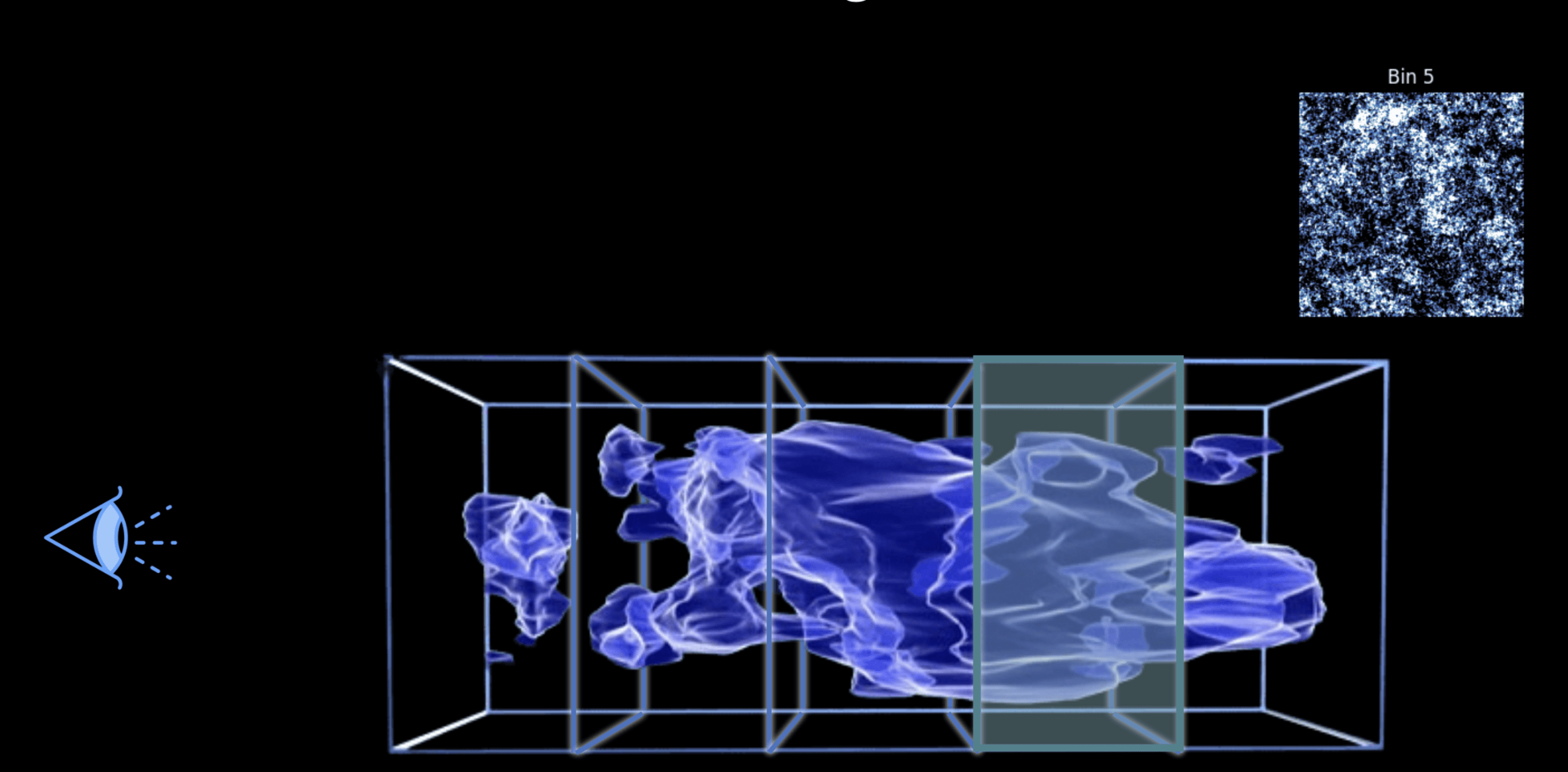
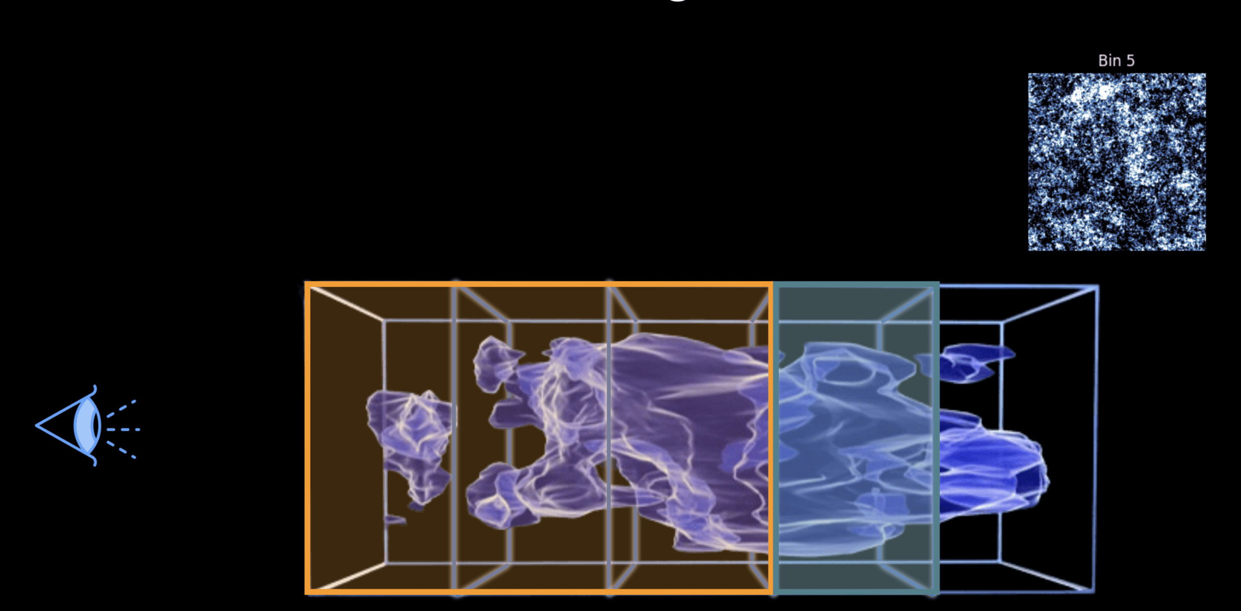
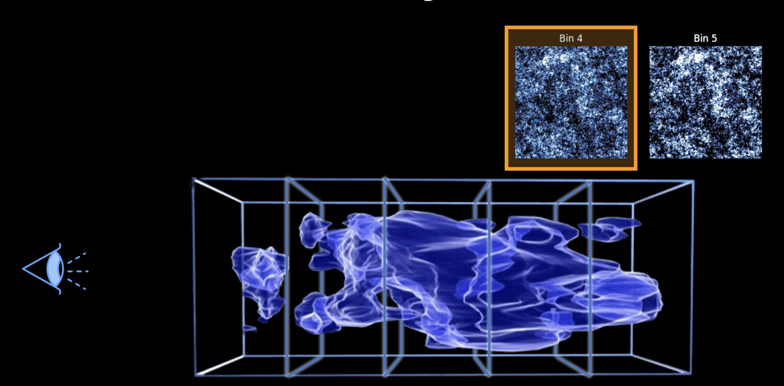
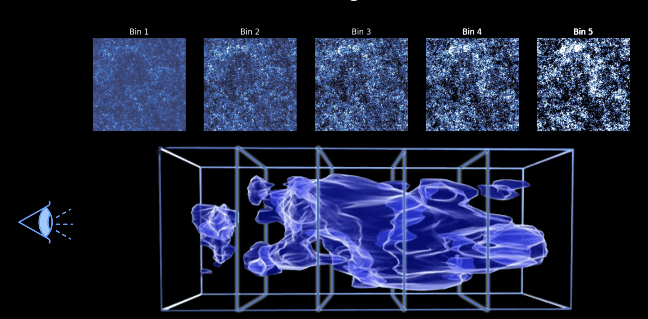
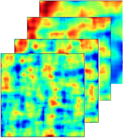
Weak lensing tomography
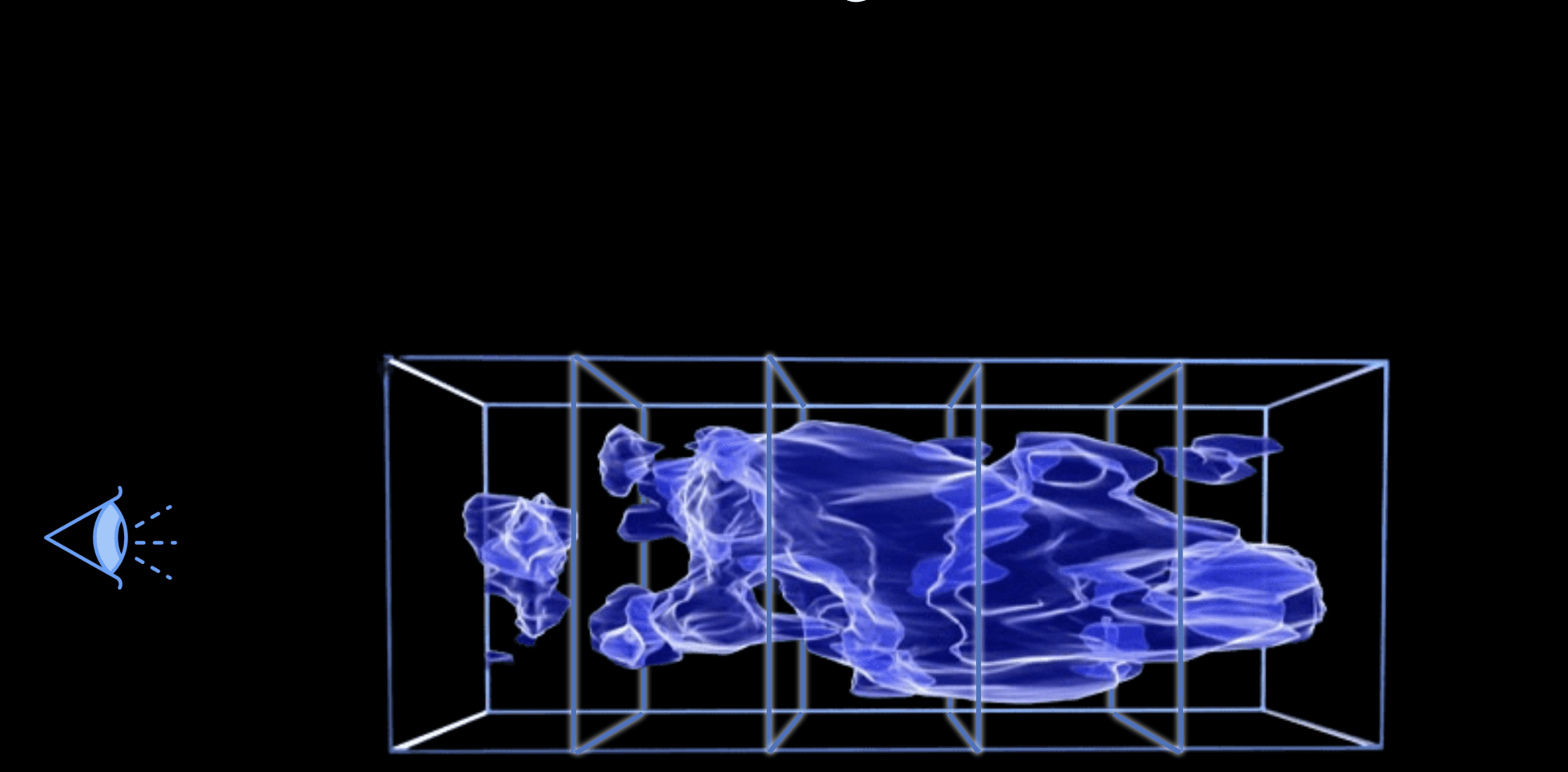
Weak lensing tomography
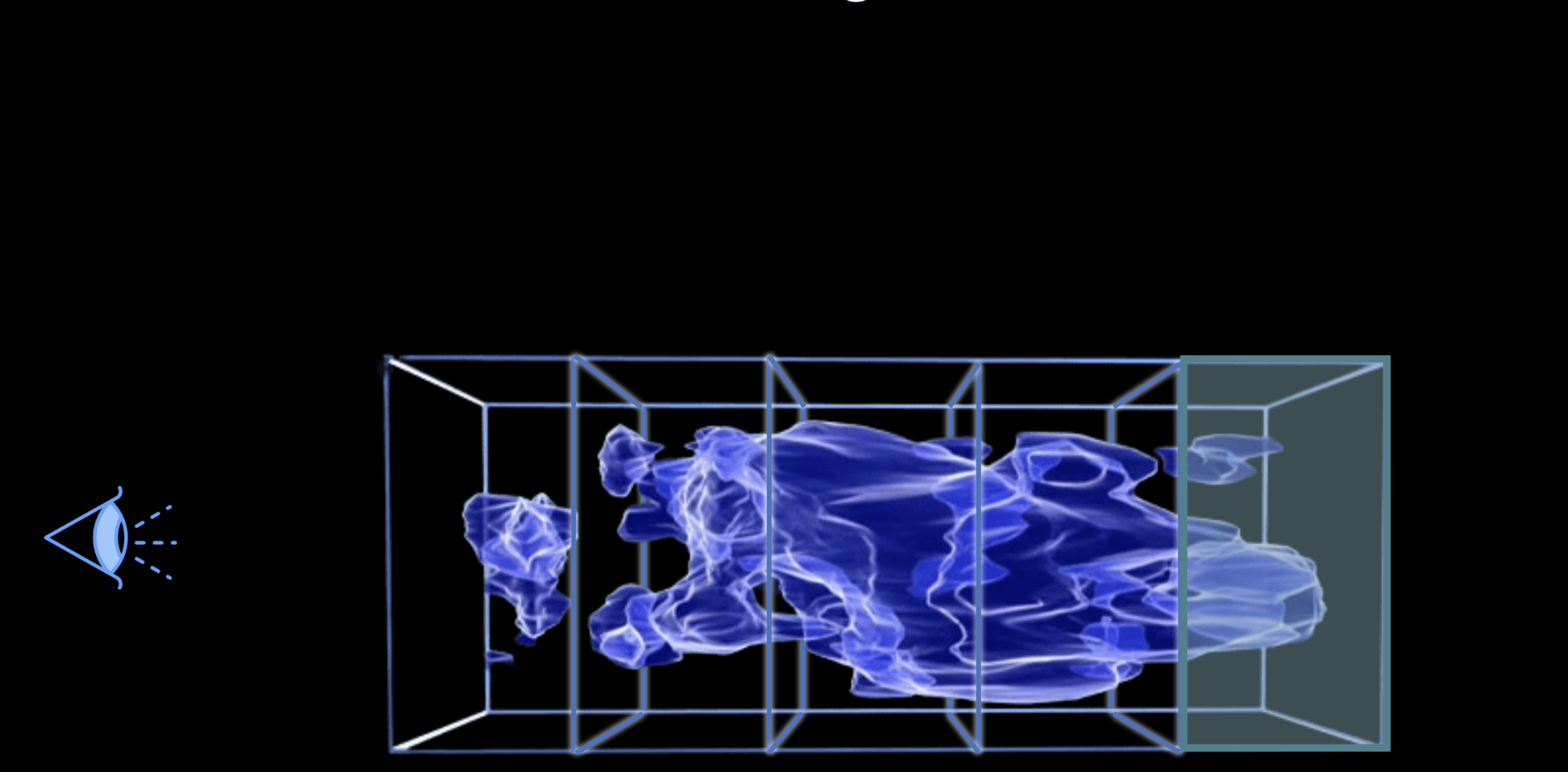
Weak lensing tomography
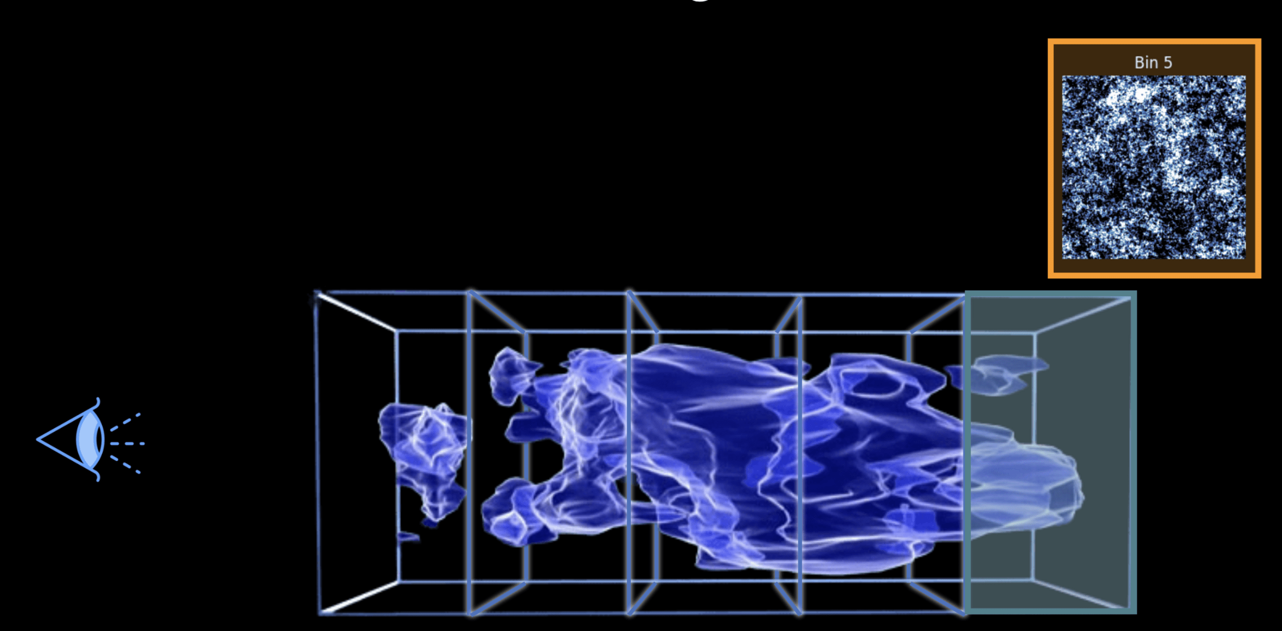
Weak lensing tomography
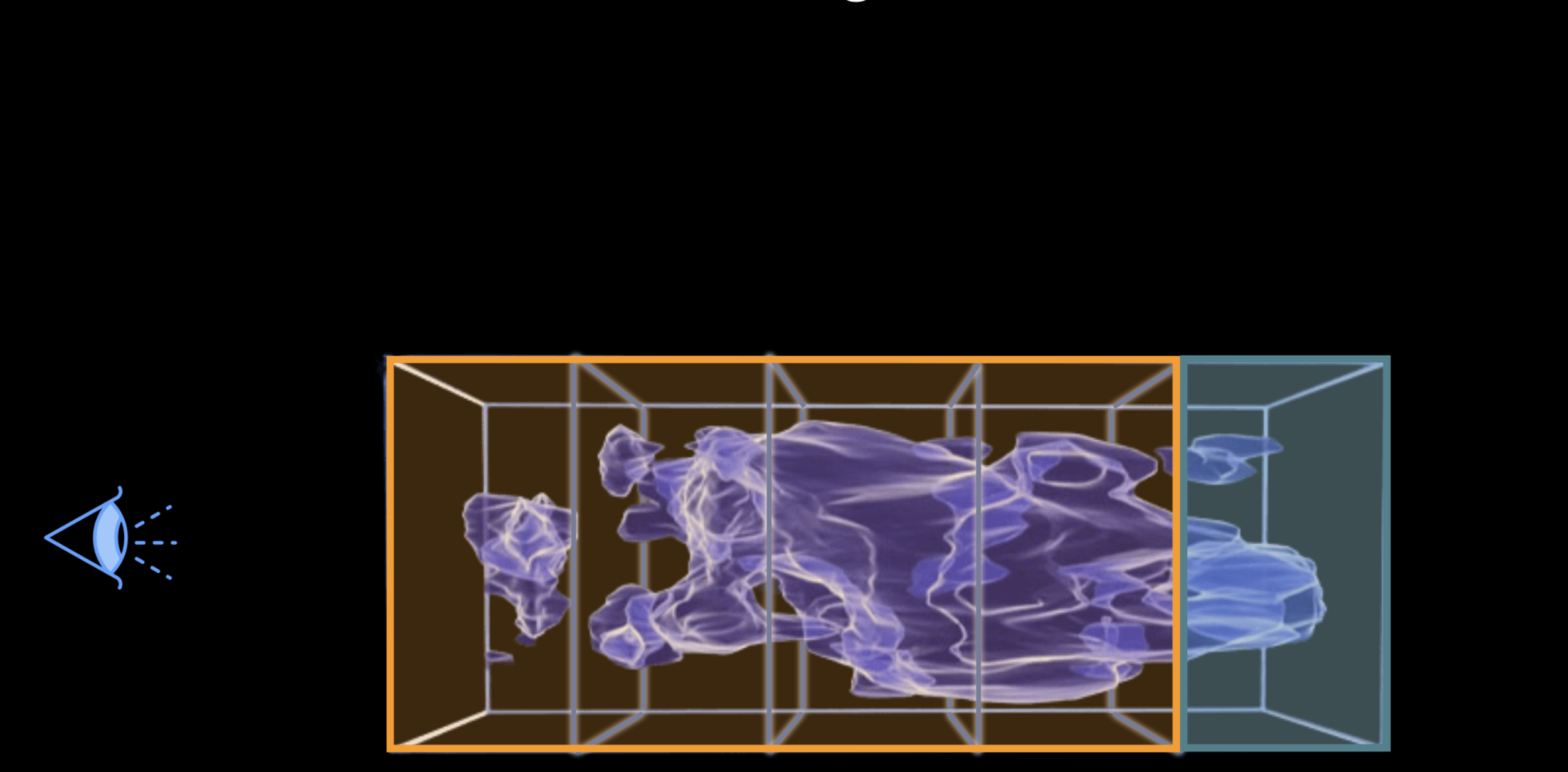
Weak lensing tomography
Weak lensing tomography
Weak lensing tomography
Weak lensing tomography
Weak lensing tomography
BNT transform
- When we observe shear, contributions come from mass at different redshifts.
- BNT Transform: method to “null” contributions from unwanted redshift ranges.
- It reorganizes weak-lensing data so that only specific redshift ranges contribute to the signal.
- BNT aligns angular (ℓ) and physical (k) scales.
- This could help mitigate baryonic effects by optimally removing sensitivity to poorly modeled small scales and controlling scale leakage.


BNT maps
no BNT
BNT


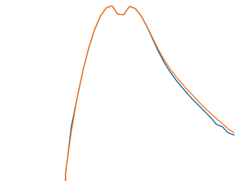
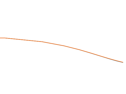
How are statistics impacted?


Power Spectrum
l1-norm
* This could help mitigate baryonic effects by optimally removing sensitivity to poorly modeled small scales and controlling scale leakage?
The Scaling of Baryonic Bias with Survey Area
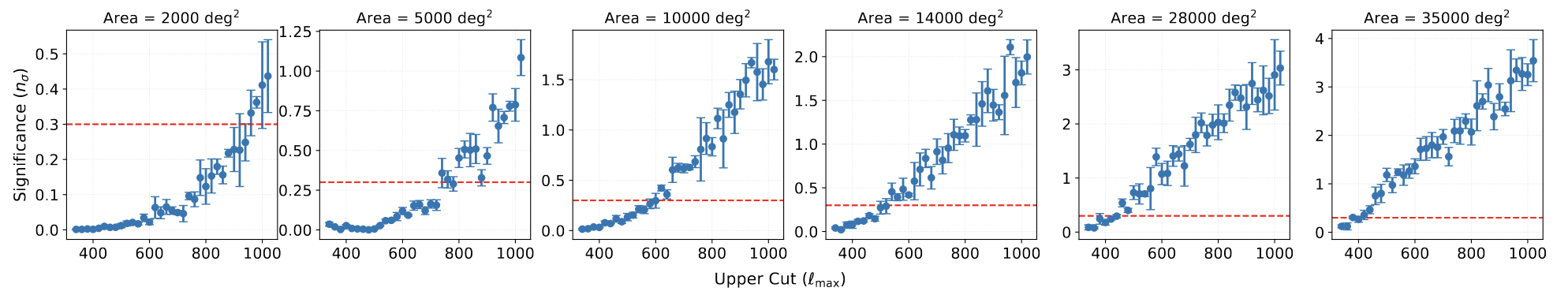
Determining Robust Scale Cuts
Information Content at Large Scales
Results
+ Benchmarking Theoretical Wavelet l1-Norm Predictions Against Cosmological Simulations
+ Euclid Key Paper: DR1 analysis with theory-based HOS
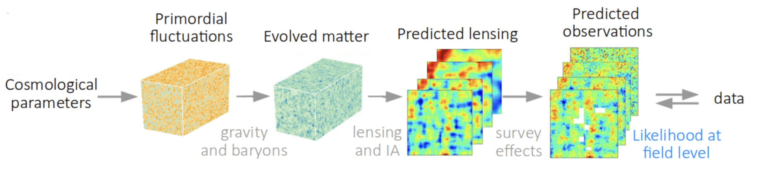
Why Field-Level Inference?
Unifying Reconstruction, Systematics, and Cosmology
\delta_{\rm IC}
\gamma_{\rm Obs}
Explicit & Lossless
-
Zero Compression: Inference directly on the pixel-level data.
-
FLI targets the full high-dim posterior.
Reconstructing ALL Latent Variables
- Beyond θcosmo reconstruct the entire formation history.
-
Initial Conditions (ICs)
-
Evolved DM Distribution
-
Peculiar Velocities
FLI Advantages:
-
Self-Consistent Systematics: Modeling noise/masks + forward model other effects physically in 3D (cosmology + systematics become part of one model, which we can sample).
-
Interpretability: analyzing stat errors directly in data space
-
Signals mix less → model misspec. easier to detect
-
Validation: Posterior Predictive Tests & Cross-Correlations (e.g., kSZ, X-ray) without CV.
-
Discovery: A platform to test physics at the field level.
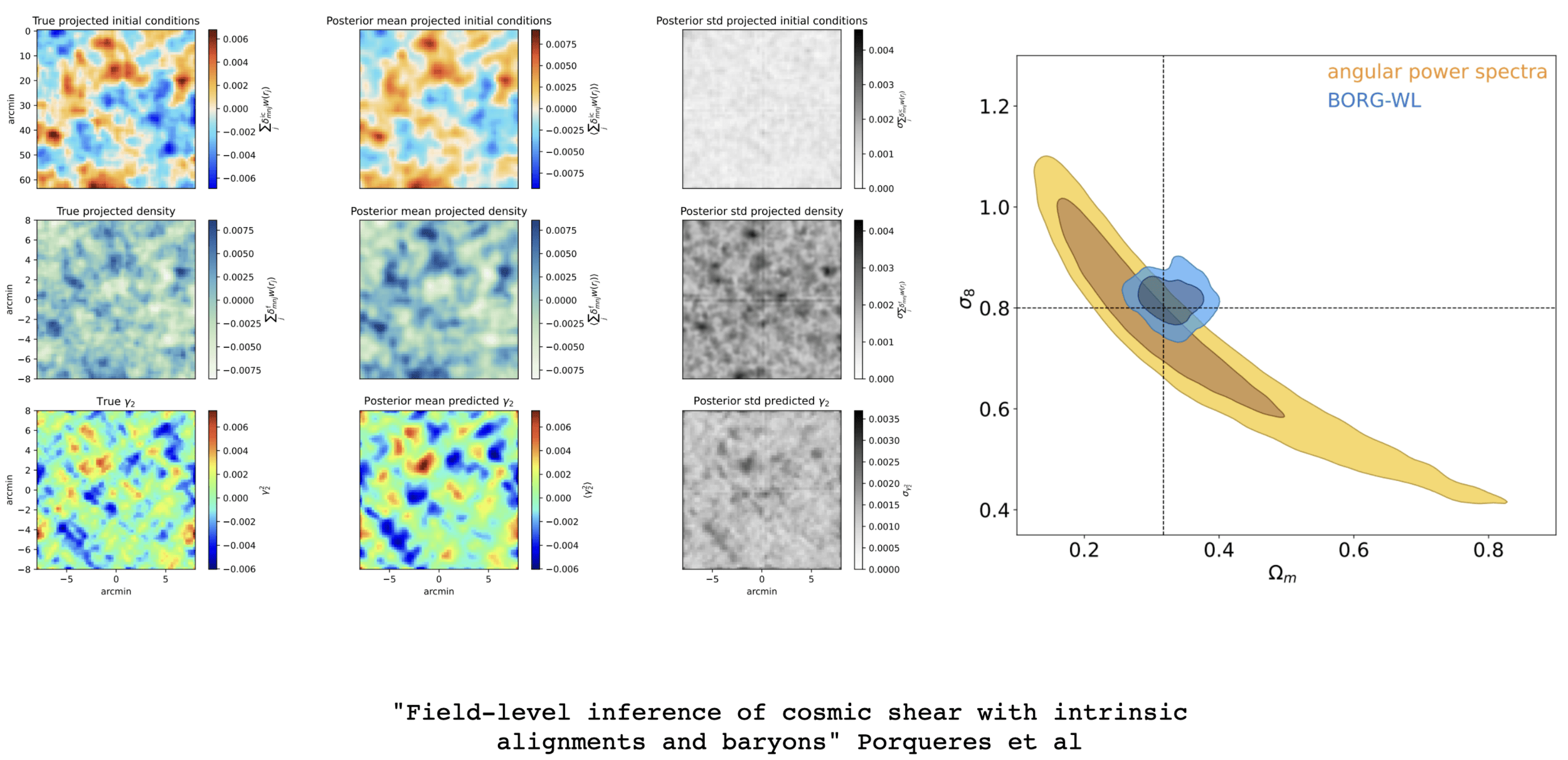
FLI for Cosmic Shear
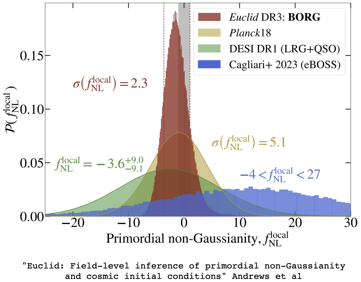
FLI for Primordial Non-Gaussianity
\theta_{\rm cosmo}
\theta_{\rm cosmo}
\theta_{\rm cosmo}
Gravity solver
Baryonification
Lensing+IA
Survey effects & systematics
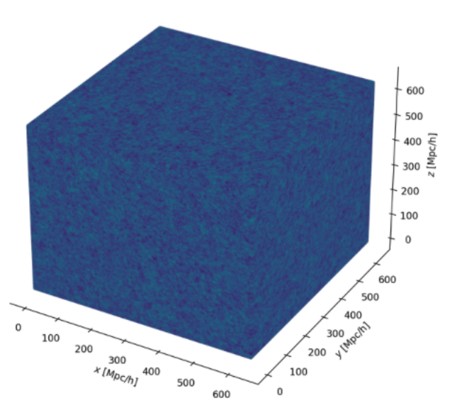
Initial conditions
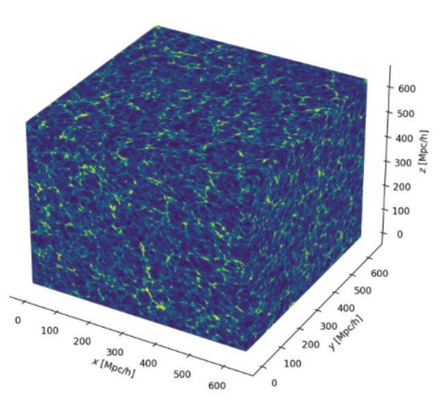
Evolved density
DM+baryons
Lensing maps
Predicted observations
Part 1: Gravity Solver
Goal: a differentiable, scalable gravity backbone that unlocks nonlinear information without bias.
Challenges:
-
Computational efficiency
- Scale to Euclid/LSST volume (Gpc)
- Resolve smaller (non-linear) scales (kpc)
- Differentiability at scale: stable gradients for HMC, memory/communication
\}
Big dynamic range
Scalability + resolution → use fully non-linear, distributed (multi-GPU) PM simulations
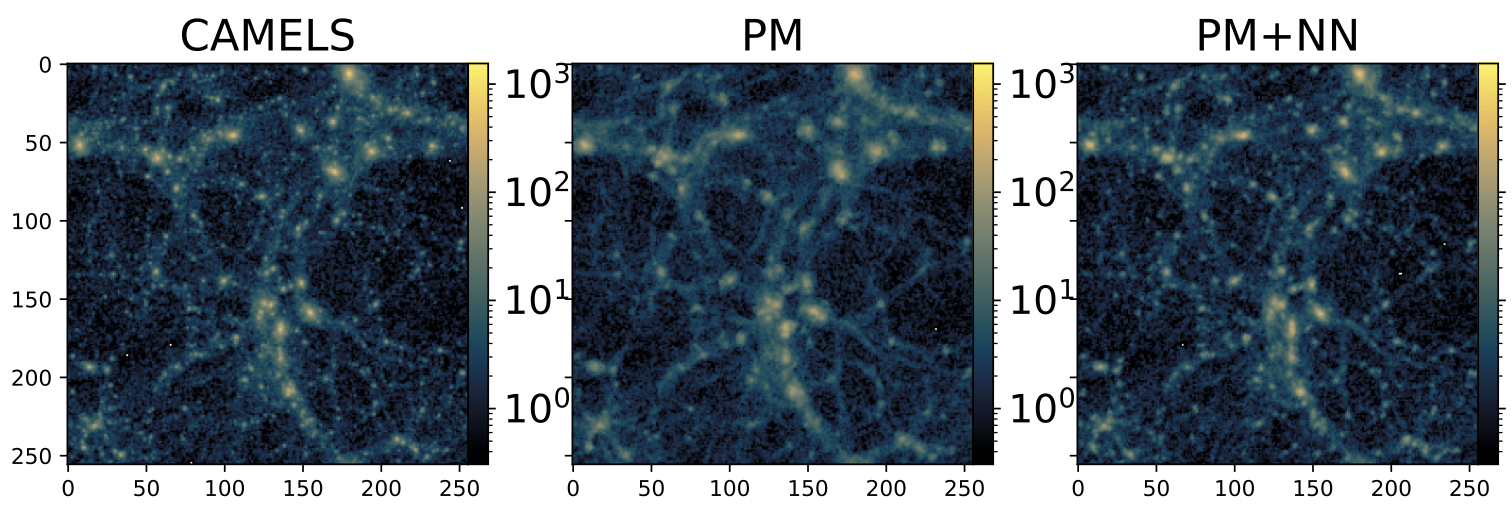
Solution: A Hybrid Physical-Neural Approach

JaxPM + jaxdecomp + jax-healpy
3D domain decomposition and distributed FFTs
Use FNO instead
- Performs global convolutions in Fourier space, learning the underlying continuous operator → learn effective Green’s function of the Poisson eqn from the data
- Captures the non-local tidal deformations
- Can distinguish between different cosmic environments
- Resolution Invariant: learned on small, high-res boxes → Zero-shot deployment on big lightcone mesh without retraining.
Computational efficiency
Resolution independence: Neural operators can generalize across resolutions after single-
scale training, facilitating multi-resolution analysis strategies
For field-level inference, we need correct velocities and displacement histories, not just final density fields. Therefore, the advanced version of my proposal is to implement Active Neural Force Correction. We inject the neural network inside the time-integration loop to correct the PM forces at every step.
-
Run Coarse PM, but at every time step, call an FNO to predict the "Residual Force" (Exact Force - PM Force) and kick the particles.
-
FNO learns the mapping
between function spaces (the density field 𝜌 to the displacement potential 𝜓 )
F_\theta(\mathbf{x}, a)=\frac{3 \Omega_m}{2} \nabla\left[\phi_{P M}(\mathbf{x}) * \mathcal{F}^{-1}\left(1+f_\theta(a,|\mathbf{k}|)\right)\right]
"Hybrid Physical Neural ODEs for Fast N-body simulations" Lanzieri, Lanusse, StarckPM solvers still face a resolution bottleneck
(mesh grid → smooths out gravity)
Strategy: inject neural correction into time-integration loop to recover small scales
Learned Isotropic Fourier Filter
predict the complex 3D force field from density, instead of just modifying potential
\theta_{\rm cosmo}
Gravity solver
Baryonification
Lensing+IA
Survey effects & systematics
Initial conditions
Evolved density
DM+baryons
Lensing maps
Predicted observations
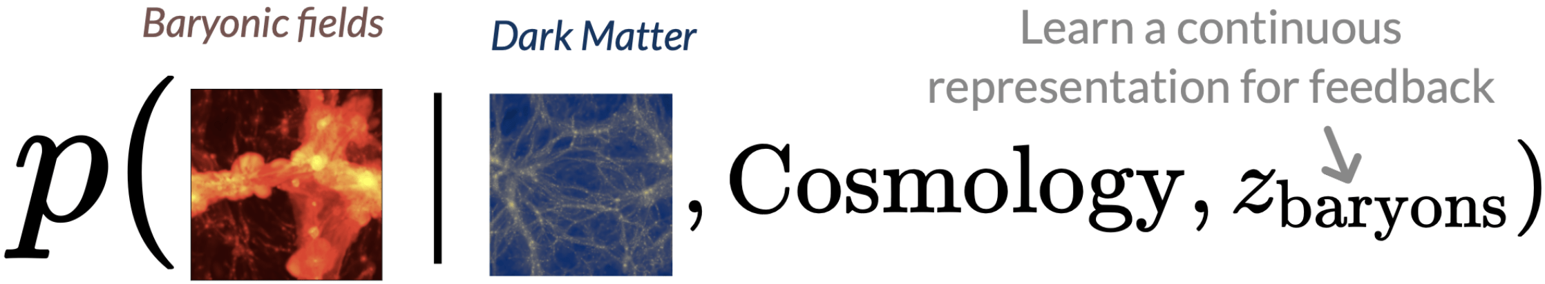
Part 2: Baryon Modeling
Challenge:
- More accurate modeling of baryons beyond simple thermodynamics
- Scalable/Fast enough for FLI + differentiable
In BORG-WL → EDG
- Displaces particles to minimize enthalpy assuming a simple polytropic eqn of state.
- It cannot create features that don't exist in the potential (e.g., AGN bubbles, non-local feedback effects).
Conditional Optimal Transport Flow-Matching (Kerrigan et al., 2024)
- The Bridge: Evolve directly from DM → Gas.
- Conditioned on Cosmology & the IC (paired datasets)
- Learns the optimal transport map from gravity solver output to hydro density fields.
- Captures non-linear feedback morphology that simple EOS models may miss.
- Reproduces the correct HOS of the gas distribution.
Baryon Emulator
PM Density
Velocity
Density
Temperature
"BaryonBridge: Interpolants models for fast hydrodynamical simulations" Horowitz et al. 2025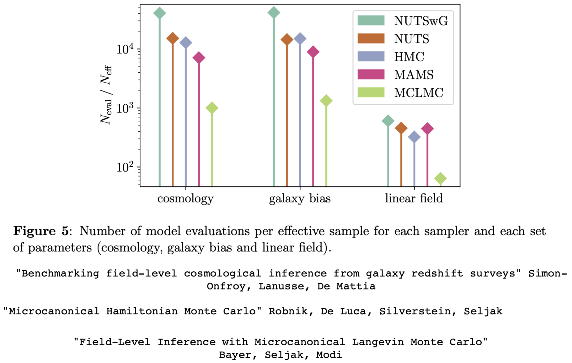
Part 3: Sampling methods
Scalable posterior exploration in high-dim spaces
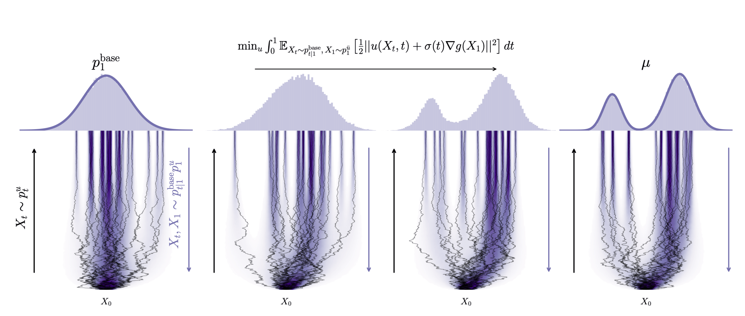
\mathcal{L}(\theta)=\mathbb{E}\left[\left\|u_\theta\left(X_t, t\right)-\left(\frac{X_1-X_t}{1-t}-\nabla E\left(X_1\right)\right)\right\|^2\right]
(unadjusted) MCLMC for scaling to ≥10^6 dim
"Adjoint Sampling: Highly Scalable Diffusion Samplers via Adjoint Matching", Havens et al.- Augment sampling with learned proposal distribution via NFs
- Flow Matching to learn probability path between prior and posterior integrated into a MCLMC/Annealed HMC loop
- provide high-fidelity proposal distributions, significantly accelerating convergence
Diffusion samplers >1 energy evaluations
per gradient update
Amortizes the cost of the forward model can perform hundreds of cheap network updates for every single expensive simulation
Adjoint Sampling learns directly from the energy function and its gradient, without requiring many data samples (many grad updates/sample
Part 4: Pixel-Level Forward Modeling
Foundation models
-
To reuse & share prior models, build flexible model, capable of modeling different types of data
-
Diff. models from corrupted data using an Expectation-Maximization approach
- Multimodal generative models to learn both from imaging & spectroscopy
- More info in latent space to improve the galaxy characteristics measurement
-
Foundational data-driven prior models → adapt to different desired populations at inference time, and can be used for many types of observations.
End-to-end diff/ble shear forward model
- Integrate detection, deblending, shear estimation, robustness to image defects.
- Denoising diffusion model priors over galaxy morphologies → optimize the posterior + sample
- Inferred population-level distributions of galaxy properties, and individual galaxy shapes jointly from the pixel data.
Combine multi-band, multi-instrument data to produce consistent UQ and posterior samples for each object.
t=T
t=0
\theta_{\rm cosmo}
Gravity solver
Baryonification
Lensing+IA
Survey effects & systematics
Initial conditions
Evolved density
DM+baryons
Lensing maps
Predicted observations
Part 6: Field Level Systematics
Exploiting Phase Information to Distinguish Physics from Artifacts → Euclid realism
- In power spectra, systematics often mimic cosmological signals.
-
In the 3D field, they possess distinct spatial signatures.
-
By differentiating through the forward model, the inference engine uses phase information to separate signal from noise.
-
Inject systematics directly into the pipeline:
- IA → TATT
- Spatially varying shear bias and survey depth
- Survey Geometry
-
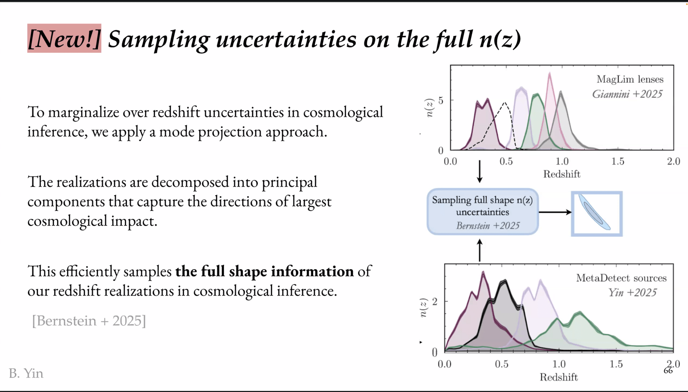
Photo-z:
-
BHM to sample n(z) and marginalise over redshift uncertainties, using forward model of the photometric fluxes
-
Part 4: Validation and Scientific Discovery
Challenge: No Clear Baseline
-
Power spectra are necessary but not sufficient.
-
First step → use HOS
-
No standard "baseline" in the literature for field-level accuracy.
-
Validation must move from statistical to mechanistic.
Test: "Do We Get the Positions Right?"
-
Input: Euclid Weak Lensing (Shear) → Reconstructed DM Field.
-
Posterior Predictive Checks:
-
Individual Objects: Turn specific clusters/voids into cosmological probes.
-
Cross-Correlation: Check alignment with tSZ/X-ray/CMB lensing.
-
If our reconstruction places a massive halo at (x,y,z), X-ray telescopes should see hot gas there.
-
Discovery & Survey Design
-
Cosmic Variance Cancellation: Inferred ICs → Deterministic prediction of all other observables.
-
Targeted Follow-Up: Use the Digital Twin to guide observations.
-
Survey Optimization: Use the reconstructed field to design optimal masks or scan strategies for future follow-ups.
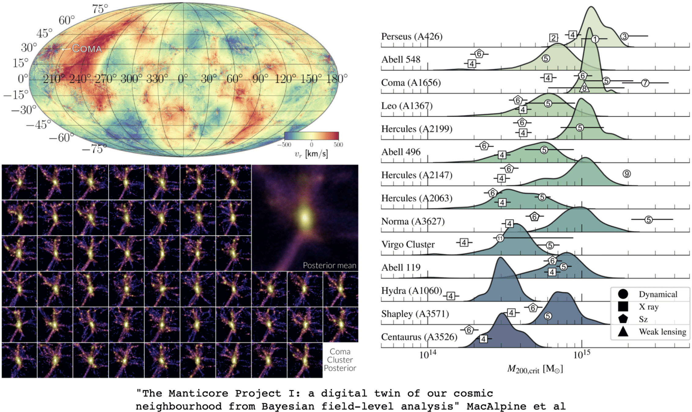
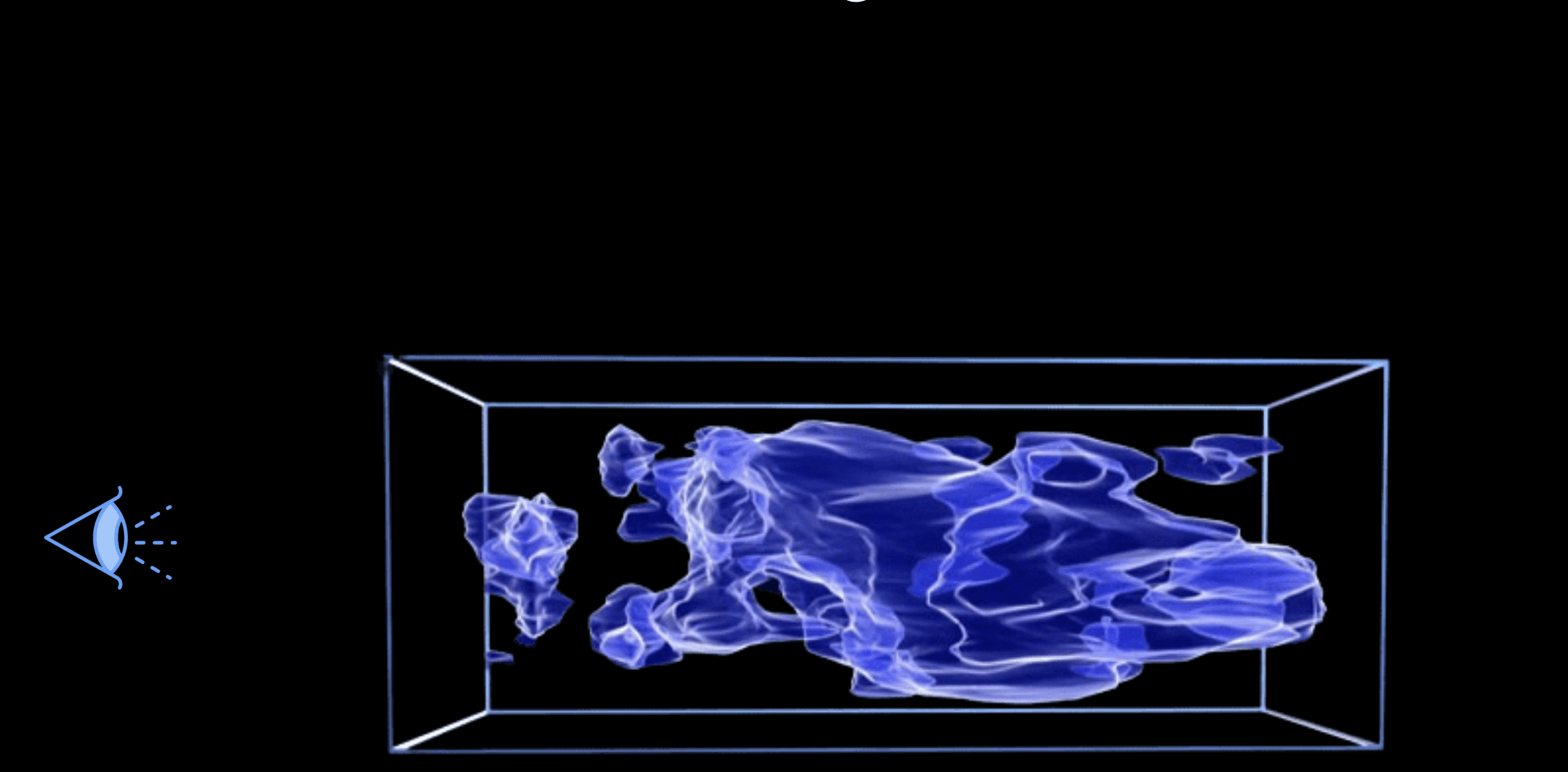
The Local Universe without CV
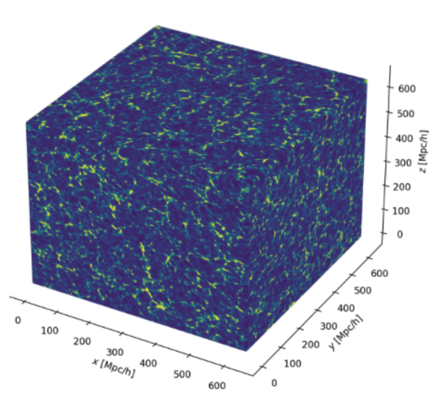
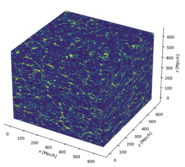
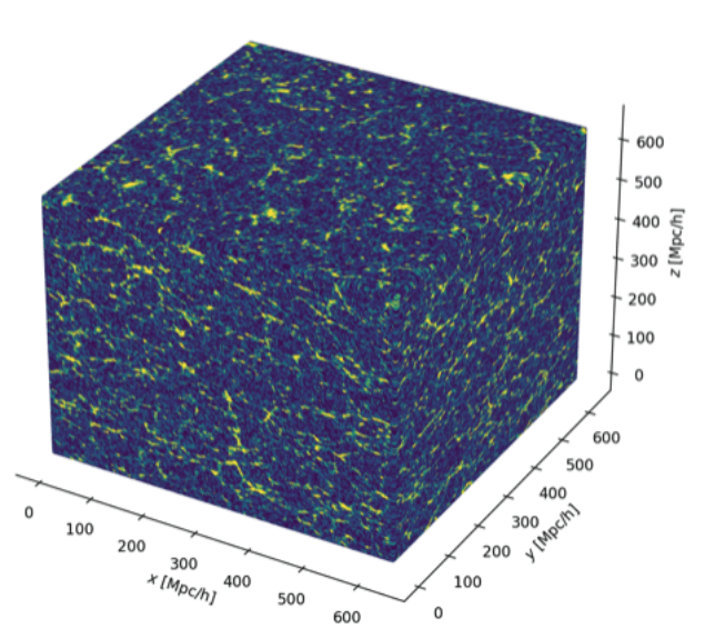
Lensing with JaxPM
JAX-Based Full Field forward model :
-
What has been done so far :
-
A fully differentiable and distributed matter only simulator using JaxPM and jaxDecomp
-
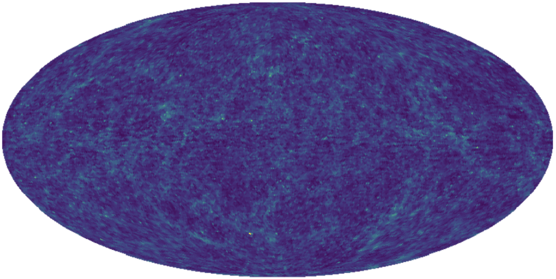
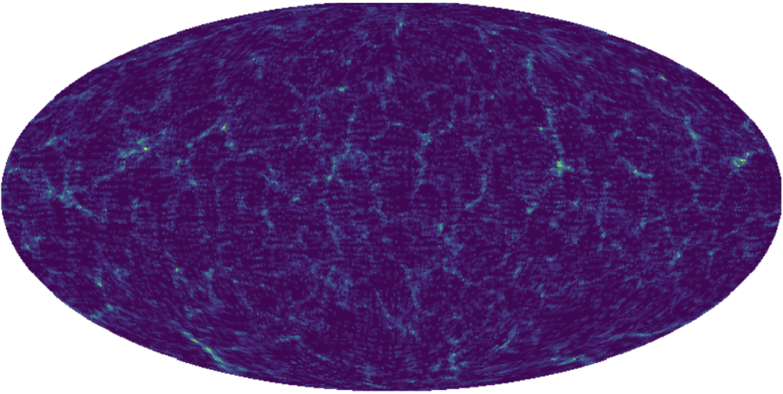
An accurate Born lensing and spherical projection that can produce convergence maps from particle mesh snapshot
-
A distributed probabilistic forward model that can be sampled with a big simulation
TODOS:
-
Have a first test on mock convergence maps with a distributed 8 GPUs forward model
-
Integrate s2fft in the pipeline to go to shear maps
AstroDeep
By Andreas Tersenov


